COMSOL 6.4 - Fresnel Rhomb

The uncoated Fresnel rhomb is one of the simplest devices for manipulating the polarization of light. In this example a Fresnel rhomb is constructed so that linearly polarized light at a specific angle of incidence becomes circularly polarized.

Reflection and Refraction of Light at Material Discontinuities

To quantify the phase delays introduced by total internal reflection within a glass prism, a preliminary understanding of the fundamentals of reflection and refraction of light is required. The following is explained in more detail in Ref. 1 and in the Ray Optics Module User’s Guide.

When a ray of light reaches the boundary between two dielectric media, a refracted ray is released in a direction determined by Snell’s law,

(1)

where

•

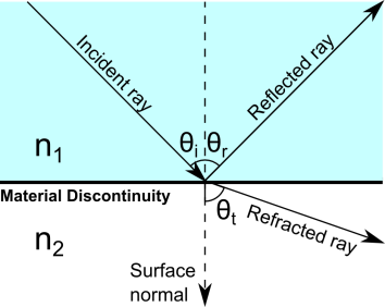
n1 (dimensionless) is the refractive index of the medium containing the incident ray,

•

n2 (dimensionless) is the refractive index of the medium containing the refracted ray,

•

θi (SI unit: rad) is the angle of incidence, and

•

θt (SI unit: rad) is the angle of refraction.

Alternatively, Snell’s law may be written as

(2)

which shows that the direction cosine of the refracted ray is either a pure real number or a pure imaginary number when the refractive indices are real.

In addition to the refracted ray described above, a reflected ray is released with an angle of reflection equal to the angle of incidence. The incident ray, reflected ray, refracted ray, and surface normal all lie within the same plane, called the plane of incidence. These angles are illustrated below.

Figure 1: Incident, reflected, and refracted rays at an interface between two materials of different refractive indices.

The electric field amplitudes of the reflected and refracted rays are related to the amplitude of the incident ray by the Fresnel Equations:

(3)

(4)

where

•

the subscript p (for “parallel”) represents the electric field component parallel to the plane of incidence,

•

the subscript s (from the German “senkrecht”, or “perpendicular”) represents the electric field component perpendicular to the plane of incidence,

•

the superscript (i) represents the incident ray,

•

the superscript (r) represents the reflected ray, and

•

the superscript (t) represents the refracted ray.

The variables r and t are called the reflection coefficient and transmission coefficient, respectively. For example, rp is the reflection coefficient of p-polarized radiation, or radiation polarized so that the electric field vector lies in the plane of incidence.

The ratio of the intensities of the transmitted and reflected rays to the intensity of the incident ray are called the transmittance T and reflectance R, respectively, given by

(5)

(6)

By substituting the definitions of the Fresnel coefficients for either s- or p-polarized radiation into Equation 5 and Equation 6, one obtains R + T = 1.

If the ray is propagating from a medium of higher refractive index to a medium of lower refractive index, that is, n2 < n1, then there exists a maximum value of the angle of incidence, beyond which no real value of the angle of refraction exists. This is the critical angle θc, given by

(7)

which is also the angle at which the radicand in Equation 2 equals zero. When the angle of incidence is greater than the critical angle, that is, θi > θc, the ray is completely reflected and no refracted ray can propagate in the adjacent domain. This phenomenon is called total internal reflection. Because θi > θc, it follows from Equation 2 that cos θt has a value on the purely imaginary axis in the complex plane. The choice of whether to use the positive or negative imaginary value for cos θt depends on the sign convention used to write the electromagnetic wave equation; the convention used in the COMSOL optics products would require cos θt to be a negative imaginary number,

(8)

Substitution of Equation 8 into Equation 4 yields

Let n = n2 / n1; then further simplification yields

(9)

Both rp and rs are complex numbers of the form A(A∗)−1, where A is the numerator. Each numerator can be expressed in terms of polar coordinates in the complex plane,

where the phases are

(10)

so that the reflection coefficients are of the form

(11)

which confirms that both reflection coefficients have unit magnitude during TIR.

Let δp and δs be the arguments of the complex-valued quantities rp and rs, respectively,

(12)

Comparing Equation 11 with Equation 12 and substituting the expressions in Equation 10 then yields

(13)

The phase delay introduced by the total internal reflection is the difference between the two arguments,

Using the difference identity

and substituting Equation 13 yields an expression for the phase delay,

(14)

Equation 14 is an expression for the phase delay that does not depend on the vacuum wavelength, and therefore can be considered an achromatic phase shifter if the frequency dependence of the refractive index is neglected. However, most common optical materials do not have sufficiently large refractive indices to induce a 90° phase shift with a single reflection. For example, if the region surrounding the prism is an air or vacuum domain (n2 = 1), then the smallest real value of the refractive index is approximately n1 = 2.414 for an angle of incidence of about θi = 32.9°. If the angle of incidence is 45° or greater, then no real finite value of n2 yields a 90° phase delay.

A workaround is to subject the light to multiple total internal reflections, each of which causes a smaller phase delay. In a Fresnel rhomb, light undergoes total internal reflection twice while passing through a glass prism. The Fresnel rhomb is designed and oriented so that each reflection causes a phase delay of 45°, so that the total phase delay for light passing through the prism is 90°.

Model Definition

The model geometry is an uncoated glass prism of refractive index n1 = 1.51 surrounded by air (n2 = 1). The model uses two physics interfaces and two studies.

The first physics interface is an instance of the Global ODEs and DAEs interface. This interface is used to solve Equation 14 for the angle of incidence that causes a phase retardation of δ = 45º between the s- and p-polarized components during each total internal reflection for the refractive index ratio n = 1/1.51.

The second physics interface is an instance of the Geometrical Optics interface, which is used to trace the path of a light ray through the Fresnel rhomb. The light ray enters the prism so that it undergoes total internal reflection at the angle of incidence computed by the Global ODEs and DAEs interface. The released ray is linearly polarized with its direction of polarization at a 45º angle to the plane of incidence.

The Stokes parameters are computed along each ray trajectory. These Stokes parameters can be used to describe the degree to which a ray is linearly or circularly polarized. In addition, it is possible to draw polarization ellipses along a plot to indicate the polarization state at discrete optical path length intervals along the ray.

Results and Discussion

The Global ODEs and DAEs interface was used to solve Equation 14 for the angle of incidence θi given the refractive index ratio n = 1/1.51 and the desired phase delay per reflection δ = 45º. The resulting value of θi is 0.84855 radians or about 48.618°.

The computed value of θi was then used in the geometry setup of the Fresnel rhomb, which is simply a parallelogram extruded into a 3D geometry.


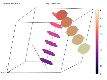
	The Stokes parameters are also computed along the ray paths in 2D geometries, so in principle the Fresnel rhomb could instead be modeled in 2D. However, in 3D it is easier to visualize the state of ray polarization because the 3D Ray Trajectories plot includes a built-in option to display polarization ellipses along the ray trajectories.

The default plot is shown in Figure 2. The color expression shows the optical path length along the ray. The circles and ellipses along the ray path are polarization ellipses that indicate the state of polarization. The arrows on the perimeter of each circle or ellipse indicate the sense of rotation of the instantaneous electric field vector. The ray enters the prism from the left side of the image. After one total internal reflection the ray becomes elliptically polarized. After two total internal reflections the polarization ellipses appear circular.

The degree of circular polarization can be quantified by plotting the ratio of the fourth and first Stokes parameters. The first Stokes parameter is the ray intensity; the fourth Stokes parameter is the degree of circular polarization. A more detailed discussion of Stokes parameters and polarization is given in the Ray Optics Module User’s Guide.

The ratio of the Stokes parameters is plotted in Figure 3. Initially the ratio is zero, meaning that the incident ray is linearly polarized or unpolarized. After one total internal reflection the ratio is

; values with magnitude between zero and one indicate varying degrees of elliptical polarization. After two reflections, the magnitude is approximately unity, corresponding to circular polarization.

Figure 2: Ray propagation in a Fresnel rhomb. The color expression shows the optical path length. Polarization ellipses are shown along the ray path.

Figure 3: The ratio of the fourth and first Stokes parameters is plotted as a function of optical path length.

References

1. M. Born and E. Wolf, Principles of Optics, 7th ed., Cambridge, 1999.

2. R.J. King, “Quarter-wave retardation systems based on the Fresnel rhomb principle,” J. Sci. Instrum.,vol. 43, no. 9, p. 617, 1966.

Ray_Optics_Module/Prisms_and_Coatings/fresnel_rhomb

Modeling Instructions

From the menu, choose .

New

In the window, click

Model Wizard

In the window, click

The first part of the model involves solving for the correct angle of incidence such that the Fresnel rhomb induces a 90-degree phase delay between the s- and p-polarized components of the ray.

In the tree, select > > .

Click .

Click

In the tree, select > .

Click

Global Definitions

Parameters 1

In the window, under click .

In the window for , locate the section.

In the table, enter the following settings:


Name	Expression	Value	Description
delta	45[deg]	0.7854 rad	Phase delay between s- and p-polarizations
n1	1	1	Refractive index, air
n2	1.51	1.51	Refractive index, glass
n12	n1/n2	0.66225	Refractive index ratio

The specified phase delay of 45 degrees, when applied at two surfaces, should convert linearly polarized light to circularly polarized light.

Global ODEs and DAEs (ge)

Global Equations 1 (ODE1)

Set up the interface following Equation 14.

In the window, under > click .

In the window for , locate the section.

In the table, enter the following settings:


Name	f(u,ut,utt,t) (1)	Initial value (u_0) (1)
thetai	cos(thetai)*sqrt(sin(thetai)^2-n12^2)/sin(thetai)^2-tan(delta/2)	45[deg]

Study 1

In the toolbar, click

Results

Global Evaluation 1

In the window for , click

Table 1

Go to the window.

The resulting value is the angle of incidence, in radians, that will induce a 45-degree phase delay between s- and p-polarized light during total internal reflection. It should be approximately 0.84855.

Global Definitions

Parameters 1

In the window, expand the > node, then click > .

In the window for , locate the section.

In the table, enter the following settings:


Name	Expression	Value	Description
theta	0.84855[rad]	0.84855 rad	Angle of incidence

Alternatively, copy the numeric value from Table 1 and paste it into the column.

Geometry 1

Work Plane 1 (wp1)

In the toolbar, click

Work Plane 1 (wp1) > Plane Geometry

In the window, click .

Work Plane 1 (wp1) > Polygon 1 (pol1)

In the toolbar, click

In the window for , locate the section.

In the table, enter the following settings:


xw (m)	yw (m)
0	0
1	0
cos(theta)+1	sin(theta)
cos(theta)	sin(theta)

Click

Extrude 1 (ext1)

In the window, under > right-click and choose .

In the window for , click

Add Physics

In the toolbar, click

to open the window.

Go to the window.

In the tree, select > > .

In the section, clear the checkbox next to , which is not compatible with the Geometrical Optics interface.

Click the button in the window toolbar.

In the toolbar, click

to close the window.

Add Study

In the toolbar, click

to open the window.

Go to the window.

Find the subsection. In the tree, select > > .

In the section, clear the checkbox next to , which will not be solved for in the second study.

Click the button in the window toolbar.

In the toolbar, click

to close the window.

Materials

Glass

In the toolbar, click

In the window for , type Glass in the text field.

Locate the section. In the table, enter the following settings:


Property	Variable	Value	Unit	Property group
Refractive index, real part	n_iso ; nii = n_iso, nij = 0	n2	1	Refractive index

Geometrical Optics (gop)

In the window, under click .

In the window for , locate the section.

In the next text field, type n1.

Locate the section. In the text field, type 0.

Locate the section. From the list, choose .

Locate the section. Select the checkbox.

Release from Grid 1

In the toolbar, click

and choose .

In the window for , locate the section.

In the qy,0 text field, type 0.5.

In the qz,0 text field, type 0.5.

Locate the section. Specify the L0 vector as


sin(theta)	x
-cos(theta)	y
0	z

Locate the section. From the list, choose .

From the list, choose .

In the a2,0 text field, type 1.

The released ray will then be linearly polarized at a 45-degree angle to the plane of incidence.

Add an antireflective coating to the surfaces where the ray enters and leaves the glass.

Material Discontinuity 2

In the toolbar, click

and choose .

Select Boundaries 1 and 6 only.

In the window for , locate the section.

From the list, choose .

Study 2

Step 1: Ray Tracing

In the window, under click .

In the window for , locate the section.

From the list, choose .

Click

In the dialog, type 0.4 in the text field.

In the text field, type 4.

Click .

In the toolbar, click

Results

Ray Trajectories (gop)

The default plot shows the path of the ray as it undergoes total internal reflection in the prism. The default color expression is the intensity, which is nearly constant because the incident ray is treated as a planar wavefront.

Ray Trajectories 1

In the window, expand the node, then click .

In the window for , locate the section.

Find the subsection. From the list, choose .

In the text field, type 15.

The default expressions are the components of the semimajor and semiminor axes of the polarization ellipse. The ellipses show that the ray is initially linearly polarized at a 45-degree angle to the plane of incidence, then becomes elliptically polarized after one reflection and circularly polarized after two.

Color Expression 1

The intensity is uniform along the ray path, so instead use the optical path length to color it.

In the window, expand the node, then click .

In the window for , click in the upper-right corner of the section. From the menu, choose > > > .

Locate the section. From the list, choose .

In the toolbar, click

Rotate the window so that the polarization ellipses of the ray can be clearly seen as it exits the prism. Click the button to get a clearer view. Then compare the resulting plot to Figure 2.

Now that the polarization ellipses have been visualized, use the Stokes parameters to confirm that the outgoing array is circularly polarized and not just elliptically polarized.

1D Plot Group 2

In the toolbar, click

In the window for , locate the section.

From the list, choose .

Click to expand the section. From the list, choose .

In the text area, type Degree of circular polarization.

Locate the section.

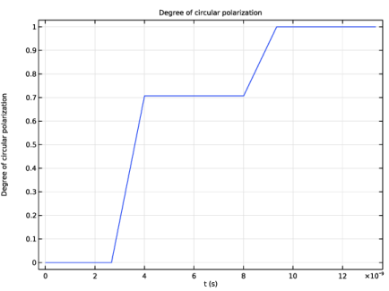
Select the checkbox. In the associated text field, type Degree of circular polarization.

Use the plot to show quantitatively how the ray becomes circularly polarized after it undergoes total internal reflection twice.

Ray 1

In the toolbar, click

and choose .

In the window for , locate the section.

In the text field, type gop.s3/gop.s0.

In this expression, gop.s3 is the Stokes parameter that indicates circular polarization, and gop.s0 is the ray intensity. The ratio of these two Stokes parameters is 1 or -1 for circularly polarized light and 0 for unpolarized or linearly polarized light.

In the toolbar, click

. Compare the resulting plot to Figure 3.