PDF

Rotating Microwave Oven with Phase Transition
Introduction
Simulating a rotating microwave oven helps us understand how microwave energy interacts with objects, affecting their internal temperature and cooking results. It also aids in refining microwave oven designs and understanding heat transfer during heating. The example model demonstrates how heat transfers within a potato as it changes from moist to dehydrated, addressing its material properties and microwave absorption rates using the phase change material feature. These factors are essential for accurately modeling cooking or heating processes.
Figure 1: Heated potato inside a rotating domain.
Model Definition
A spherical, water-rich load simulating a potato is placed on a rotating glass tray in a microwave oven, positioned off-center. A 1 kW, 2.45 GHz microwave power is applied through a waveguide feed, and the tray rotates at 9 degrees per second. The heat transfer model addresses the transition from a water-rich to a dehydrated phase, including changes in material properties and microwave losses. The simulation rotates the model in 0.25-second steps, with a mesh adjusted for conformity at each step using the Phase Change Material feature from the Heat Transfer in Solids interface and the Events interface for step-wise motion.
Electromagnetic Waves, Frequency Domain
A Port feature is configured to represent the waveguide boundary with a 1 kW power input and a rectangular port type. The Continuity feature ensures electromagnetic field continuity across boundaries, while the Wave Equation, Electric 2 feature models the lossy behavior of electric waves in the potato. It accounts for dielectric losses with temperature-dependent permittivity values.
Heat Transfer in Solids
This interface describes thermal behavior within the potato and glass plate domains. The potato domain includes a Phase Change Material feature, crucial for simulating transitions between water-rich and dehydrated states. It is configured with a phase change temperature of 373.15 K and a latent heat of 2.2564 × 106 J/kg. Thermal conductivity values are specified for each direction to model heat conduction accurately.
Moving Mesh
The model utilizes the Moving Mesh functionality to handle rotating domains. The Rotating Domain feature describes rotational motion with a parameter for the rotation angle, enabling dynamic geometry changes during rotation.
Events
The Events interface manages discrete events and state changes. An Explicit Event feature defines time-dependent changes with a period specified by dt, while the Discrete States feature tracks rotation angles and step numbers.
Multiphysics
The Electromagnetic Heating multiphysics feature couples electromagnetic effects with heat transfer, integrating the impact of electromagnetic fields on thermal processes.
Additional Settings
Discretization properties for both electromagnetic and heat transfer physics are set to Linear.
The Model Builder sets up a comprehensive multiphysics simulation integrating electromagnetic wave propagation, heat transfer, and discrete events with rotating domains under Moving Mesh functionality. This setup provides a detailed and interactive simulation of complex physical processes, considering dynamic changes in geometry and the interaction of various physical phenomena.
Results and Discussion
The average temperature in the potato, is shown in Figure 2, gradually approaches 380 K over time.
Figure 2: The average temperature in the potato over time
Figure 3 show the initial electric field norm distribution at the bottom of the microwave oven, with a relatively stronger field observed underneath the potato. Temperature distribution in the potato and glass plate domains is shown in Figure 4. The glass plate does not heat up from the electromagnetic waves. However, the area adjacent to the potato is affected due to the temperature increase from the potato.
Figure 3: A plot of the electric field norm distribution at the bottom of the microwave oven.
Figure 4: Temperature in the potato and glass domains.
Figure 5: Fraction of water rich state.
Figure 6: Fraction of dehydrate state.
Figure 5 and Figure 6 describe the fraction of water rich and dehydrate states respectively. Over the time, the bottom part of the potato heat up more than other areas and the water rich state turns into the dehydrate state.
The ratio of the coupled power to the microwave oven can be computed based on the reflection coefficient at the port that provides the excitation. Interestingly, the low coupling is observed periodically in relation to specific position of the potato, particularly when the glass plate is rotated 90 and 270 degrees from its original position (see Figure 7).
Figure 7: Coupled power to the microwave oven.
Figure 8 illustrates a variety of computed results by combining multiple plots.
Figure 8: Combination plot of the electric field norm, temperature, and fraction of water-rich state.
Application Library path: RF_Module/Microwave_Heating/rotating_microwave_oven
Modeling Instructions
From the Main Toolbar menu, choose New.
New
In the New window, click  Model Wizard.
Model Wizard
1
In the Model Wizard window, click  3D.
2
In the Select Physics tree, select Radio Frequency > Electromagnetic Waves, Frequency Domain (emw).
3
Click Add.
4
In the Select Physics tree, select Heat Transfer > Heat Transfer in Solids (ht).
5
Click Add.
6
In the Select Physics tree, select Mathematics > Deformed Mesh > Moving Mesh > Rotating Domain.
7
Click Add.
8
In the Select Physics tree, select Mathematics > ODE and DAE Interfaces > Events (ev).
9
Click Add.
10
Click  Study.
11
In the Select Study tree, select Empty Study.
12
Global Definitions
Geometry Parameters
1
In the Model Builder window, under Global Definitions click Parameters 1.
2
In the Settings window for Parameters, type Geometry Parameters in the Label text field.
3
Locate the Parameters section. Click  Load from File.
4
Simulation Parameters
1
In the Home toolbar, click  Parameters and choose Add > Parameters.
2
In the Settings window for Parameters, type Simulation Parameters in the Label text field.
3
Locate the Parameters section. In the table, enter the following settings:
Geometry 1
1
In the Model Builder window, under Component 1 (comp1) click Geometry 1.
2
In the Settings window for Geometry, locate the Advanced section.
3
From the Default repair tolerance list, choose Relative.
Block 1 (blk1)
1
In the Geometry toolbar, click  Block.
2
In the Settings window for Block, locate the Size and Shape section.
3
In the Width text field, type wo.
4
In the Depth text field, type do.
5
In the Height text field, type ho.
6
Locate the Position section. In the x text field, type -wo/2.
7
In the y text field, type -do/2.
8
Click  Build Selected.
9
Click the  Wireframe Rendering button in the Graphics toolbar.
Block 2 (blk2)
1
In the Geometry toolbar, click  Block.
2
In the Settings window for Block, locate the Size and Shape section.
3
In the Width text field, type wg.
4
In the Depth text field, type dg.
5
In the Height text field, type hg.
6
Locate the Position section. In the x text field, type wo/2.
7
In the y text field, type -dg/2.
8
In the z text field, type ho-hg.
Cylinder 1 (cyl1)
1
In the Geometry toolbar, click  Cylinder.
2
In the Settings window for Cylinder, locate the Size and Shape section.
3
In the Radius text field, type rp.
4
In the Height text field, type ho.
5
Click to expand the Layers section. In the table, enter the following settings:
6
Clear the Layers on side checkbox.
7
Select the Layers on bottom checkbox.
Difference 1 (dif1)
1
In the Geometry toolbar, click  Booleans and Partitions and choose Difference.
2
In the Settings window for Difference, locate the Difference section.
3
Click to select the  Activate Selection toggle button for Objects to add.
4
Select the objects blk1 and blk2 only.
5
Click to select the  Activate Selection toggle button for Objects to subtract.
6
7
From the Repair tolerance list, choose Automatic.
8
Select the Keep objects to subtract checkbox.
9
Click  Build Selected.
Extract 1 (extract1)
1
In the Geometry toolbar, click  Extract.
2
In the Settings window for Extract, locate the Entities or Objects to Extract section.
3
From the Geometric entity level list, choose Domain.
4
On the object cyl1, select Domain 1 only.
5
From the Input object handling list, choose Create remainder object.
Sphere 1 (sph1)
1
In the Geometry toolbar, click  Sphere.
2
In the Settings window for Sphere, locate the Size section.
3
In the Radius text field, type rpot.
4
Locate the Position section. In the x text field, type gpos.
5
In the z text field, type hp+0.0175.
Difference 2 (dif2)
1
In the Geometry toolbar, click  Booleans and Partitions and choose Difference.
2
3
In the Settings window for Difference, locate the Difference section.
4
Click to select the  Activate Selection toggle button for Objects to subtract.
5
Select the object extract1(1) only.
6
Select the Keep objects to subtract checkbox.
7
From the Repair tolerance list, choose Automatic.
Rotate 1 (rot1)
1
In the Geometry toolbar, click  Transforms and choose Rotate.
2
Select the objects dif2, extract1(1), and extract1(2) only.
3
In the Settings window for Rotate, locate the Rotation section.
4
In the Angle text field, type rot.
Union 1 (uni1)
1
In the Geometry toolbar, click  Booleans and Partitions and choose Union.
2
Select the objects rot1(1), rot1(2), and rot1(3) only.
3
In the Settings window for Union, locate the Union section.
4
From the Repair tolerance list, choose Automatic.
5
Click  Build Selected.
Form Union (fin)
1
In the Model Builder window, under Component 1 (comp1) > Geometry 1 click Form Union (fin).
2
In the Settings window for Form Union/Assembly, locate the Form Union/Assembly section.
3
From the Action list, choose Form an assembly.
4
From the Repair tolerance list, choose Relative.
5
In the Geometry toolbar, click  Build All.
Definitions
Global Variable Probe 1 (var1)
1
In the Model Builder window, expand the Component 1 (comp1) > Definitions node.
2
Right-click Definitions and choose Probes > Global Variable Probe.
3
In the Settings window for Global Variable Probe, locate the Expression section.
4
In the Expression text field, type ang/(pi/(2*N)).
5
Select the Description checkbox. In the associated text field, type Angular step number.
6
Click to expand the Table and Window Settings section. Click  Add Plot Window.
Global Variable Probe 2 (var2)
1
In the Definitions toolbar, click  Probes and choose Global Variable Probe.
2
In the Settings window for Global Variable Probe, locate the Expression section.
3
In the Expression text field, type 100[%]*(1-abs(emw.S11)^2).
4
In the Table and plot unit field, type %.
5
Select the Description checkbox. In the associated text field, type Coupled power.
6
Locate the Table and Window Settings section. Click  Add Plot Window.
Domain Probe 1 (dom1)
1
In the Definitions toolbar, click  Probes and choose Domain Probe.
2
In the Settings window for Domain Probe, locate the Source Selection section.
3
From the Selection list, choose Manual.
4
Click  Clear Selection.
5
6
Locate the Expression section. In the Expression text field, type T.
7
Select the Description checkbox. In the associated text field, type Average temperature.
8
Click to expand the Table and Window Settings section. Click  Add Plot Window.
Maximum 1 (maxop1)
1
In the Definitions toolbar, click  Nonlocal Couplings and choose Maximum.
2
Integration 1 (intop1)
1
In the Definitions toolbar, click  Nonlocal Couplings and choose Integration.
2
Identity Boundary Pair 1 (ap1)
1
In the Model Builder window, click Identity Boundary Pair 1 (ap1).
2
In the Settings window for Pair, locate the Frame section.
3
Select the Manual control of frame checkbox.
Explicit, Data Storing Domain
1
In the Definitions toolbar, click  Explicit.
2
In the Settings window for Explicit, type Explicit, Data Storing Domain in the Label text field.
3
Explicit, Data Storing Boundary
1
Right-click Explicit, Data Storing Domain and choose Duplicate.
2
In the Settings window for Explicit, type Explicit, Data Storing Boundary in the Label text field.
3
Locate the Input Entities section. From the Geometric entity level list, choose Boundary.
4
Materials
Air
1
In the Model Builder window, under Component 1 (comp1) right-click Materials and choose Blank Material.
2
In the Settings window for Material, type Air in the Label text field.
3
Click to expand the Material Properties section. Locate the Material Contents section. In the table, enter the following settings:
Glass
1
Right-click Materials and choose Blank Material.
2
In the Settings window for Material, type Glass in the Label text field.
3
4
Locate the Material Contents section. In the table, enter the following settings:
Add Material from Library
In the Home toolbar, click  Windows and choose Add Material from Library.
Add Material
1
Go to the Add Material window.
2
In the tree, select Built-in > Water, liquid.
3
Click the Add to Component button in the window toolbar.
Materials
Water rich
1
In the Settings window for Material, type Water rich in the Label text field.
2
3
Locate the Material Contents section. In the table, enter the following settings:
Add Material
1
Go to the Add Material window.
2
In the tree, select Liquids and Gases > Gases > Steam.
3
Click the Add to Component button in the window toolbar.
4
In the Home toolbar, click  Add Material to close the Add Material window.
Materials
Dehydrated
1
In the Settings window for Material, type Dehydrated in the Label text field.
Here, the domain selection is empty. However, once you specify the materials for the different phases in the Phase Change Material feature later on, it automatically manages the property assignment to the appropriate domains, reducing the need for manual domain selection.
Moving Mesh
Rotating Domain 1
1
In the Model Builder window, under Component 1 (comp1) > Moving Mesh click Rotating Domain 1.
2
In the Settings window for Rotating Domain, locate the Domain Selection section.
3
Click  Remove from Selection.
4
5
Locate the Rotation section. In the α text field, type ang.
Electromagnetic Waves, Frequency Domain (emw)
1
Click the  Show More Options button in the Model Builder toolbar.
2
In the Show More Options dialog, click  Select All.
3
4
In the Model Builder window, under Component 1 (comp1) click Electromagnetic Waves, Frequency Domain (emw).
5
In the Settings window for Electromagnetic Waves, Frequency Domain, click to expand the Discretization section.
6
From the Electric field list, choose Linear.
Port 1
1
In the Physics toolbar, click  Boundaries and choose Port.
2
3
In the Settings window for Port, locate the Port Properties section.
4
From the Type of port list, choose Rectangular.
5
In the Pin text field, type 1e3[W].
Wave Equation, Electric 2
1
In the Physics toolbar, click  Domains and choose Wave Equation, Electric.
2
3
In the Settings window for Wave Equation, Electric, locate the Electric Displacement Field section.
4
From the Electric displacement field model list, choose Dielectric loss.
5
From the ε′ list, choose User defined. In the associated text field, type 64*ht.theta1+1.
6
From the ε′′ list, choose User defined. In the associated text field, type 19*ht.theta1+1.
Multiphysics
Electromagnetic Heating 1 (emh1)
In the Physics toolbar, click  Multiphysics Couplings and choose Domain > Electromagnetic Heating.
Heat Transfer in Solids (ht)
1
In the Model Builder window, under Component 1 (comp1) click Heat Transfer in Solids (ht).
2
3
In the Settings window for Heat Transfer in Solids, click to expand the Discretization section.
4
From the Temperature list, choose Linear.
Continuity 1
1
In the Model Builder window, under Component 1 (comp1) > Heat Transfer in Solids (ht) click Continuity 1.
2
In the Settings window for Continuity, locate the Advanced section.
3
Select the Disconnect pair checkbox.
Solid 2
1
In the Physics toolbar, click  Domains and choose Solid.
2
Phase Change Material 1
1
In the Physics toolbar, click  Attributes and choose Phase Change Material.
2
In the Settings window for Phase Change Material, locate the Phase Change section.
3
In the T12 text field, type 373.15[K].
4
In the L12 text field, type 2.2564E6[J/kg].
5
Locate the Phase 1 section. From the Material, phase 1 list, choose Water rich (mat3).
6
Locate the Phase 2 section. From the Material, phase 2 list, choose Dehydrated (mat4).
7
From the k2 list, choose User defined. In the associated text field, type 1e2.
Events (ev)
In the Model Builder window, under Component 1 (comp1) click Events (ev).
Explicit Event 1
1
In the Physics toolbar, click  Global and choose Explicit Event.
2
In the Settings window for Explicit Event, locate the Event Timings section.
3
In the T text field, type dt.
4
Clear the Use consistent initialization checkbox.
5
Locate the Reinitialization section. In the table, enter the following settings:
Discrete States 1
1
In the Physics toolbar, click  Global and choose Discrete States.
2
In the Settings window for Discrete States, locate the Discrete States section.
3
Mesh 1
Mapped 1
In the Mesh toolbar, click  More Generators and choose Mapped.
Size
1
In the Model Builder window, click Size.
2
In the Settings window for Size, locate the Element Size section.
3
Click the Custom button.
4
Locate the Element Size Parameters section. In the Maximum element size text field, type c_const/2.45[GHz]/5.
5
In the Minimum element size text field, type c_const/2.45[GHz]/6.
6
In the Maximum element growth rate text field, type 2.
7
In the Curvature factor text field, type 1.
8
In the Resolution of narrow regions text field, type 0.1.
Mapped 1
1
In the Model Builder window, click Mapped 1.
2
Distribution 1
1
Right-click Mapped 1 and choose Distribution.
2
3
In the Settings window for Distribution, locate the Distribution section.
4
In the Number of elements text field, type N.
Distribution 2
1
Right-click Mapped 1 and choose Distribution.
2
3
In the Settings window for Distribution, locate the Distribution section.
4
In the Number of elements text field, type floor(N*0.8).
Copy 1
1
In the Mesh toolbar, click  Copy and choose Copy.
2
In the Settings window for Copy, locate the Dimension section.
3
From the Geometric entity level list, choose Boundary.
4
5
Locate the Destination Entities section. Click to select the  Activate Selection toggle button.
6
Copy 2
1
In the Mesh toolbar, click  Copy and choose Copy.
2
3
In the Settings window for Copy, locate the Destination Entities section.
4
Click to select the  Activate Selection toggle button.
5
Copy 3
1
In the Mesh toolbar, click  Copy and choose Copy.
2
3
In the Settings window for Copy, locate the Destination Entities section.
4
Click to select the  Activate Selection toggle button.
5
Copy 4
1
In the Mesh toolbar, click  Copy and choose Copy.
2
In the Settings window for Copy, locate the Source Entities section.
3
Click  Paste Selection.
4
In the Paste Selection dialog, type 6-13 in the Selection text field.
5
6
In the Settings window for Copy, locate the Destination Entities section.
7
Click to select the  Activate Selection toggle button.
8
Click  Paste Selection.
9
In the Paste Selection dialog, type 21, 22, 24, 25, 28-31 in the Selection text field.
10
Size 1
1
In the Model Builder window, right-click Mesh 1 and choose Size.
2
In the Settings window for Size, locate the Geometric Entity Selection section.
3
From the Geometric entity level list, choose Domain.
4
5
Locate the Element Size section. Click the Custom button.
6
Locate the Element Size Parameters section.
7
Select the Maximum element size checkbox. In the associated text field, type c_const/2.45[GHz]/sqrt(65)/5.
8
Select the Minimum element size checkbox. In the associated text field, type c_const/2.45[GHz]/sqrt(65)/6.
Free Tetrahedral 1
1
In the Mesh toolbar, click  Free Tetrahedral.
2
In the Settings window for Free Tetrahedral, click to expand the Element Quality Optimization section.
3
Find the Accept lower element quality to subsection. Clear the Avoid inverted curved elements checkbox.
4
Click  Build All.
Study 1
Step 1: Frequency–Transient
1
In the Study toolbar, click  More Study Steps and choose Time Dependent > Frequency–Transient.
2
In the Settings window for Frequency–Transient, locate the Study Settings section.
3
In the Output times text field, type range(0,0.25,100).
4
In the Frequency text field, type 2.45[GHz].
5
Click to expand the Store in Output section. In the table, enter the following settings:
6
Under Selections, click  Add.
7
In the Add dialog, in the Selections list, choose Explicit, Data Storing Domain (Domain) and Explicit, Data Storing Boundary (Boundary).
8
Solution 1 (sol1)
1
In the Model Builder window, right-click Solver Configurations and choose Show Default Solver.
2
In the Model Builder window, expand the Solution 1 (sol1) node, then click Dependent Variables 1.
3
In the Settings window for Dependent Variables, locate the Residual Scaling section.
4
From the Method list, choose Automatic.
5
In the Model Builder window, expand the Study 1 > Solver Configurations > Solution 1 (sol1) > Dependent Variables 1 node, then click Study 1 > Solver Configurations > Solution 1 (sol1) > Time-Dependent Solver 1.
6
In the Settings window for Time-Dependent Solver, click to expand the Time Stepping section.
7
From the Steps taken by solver list, choose Manual.
8
In the Time step text field, type 0.25.
9
In the Event tolerance text field, type 0.001.
10
Right-click Time-Dependent Solver 1 and choose Fully Coupled.
11
In the Settings window for Fully Coupled, locate the General section.
12
From the Linear solver list, choose Direct.
13
Click to expand the Method and Termination section. From the Nonlinear method list, choose Automatic (Newton).
14
In the Maximum number of iterations text field, type 25.
15
In the Model Builder window, click Direct.
16
In the Settings window for Direct, locate the General section.
17
From the Solver list, choose PARDISO.
18
In the Model Builder window, click Study 1.
19
In the Settings window for Study, locate the Study Settings section.
20
Clear the Generate default plots checkbox.
21
In the Study toolbar, click  Compute.
Results
Probe Plot Group 2
1
In the Model Builder window, under Results click Probe Plot Group 2.
2
In the Settings window for 1D Plot Group, locate the Legend section.
3
From the Position list, choose Lower middle.
Probe Plot Group 3
1
In the Model Builder window, click Probe Plot Group 3.
2
In the Settings window for 1D Plot Group, locate the Legend section.
3
From the Position list, choose Lower middle.
Probe Plot Group 4
1
In the Model Builder window, click Probe Plot Group 4.
2
In the Settings window for 1D Plot Group, locate the Legend section.
3
From the Position list, choose Lower middle.
Electric Field (emw)
1
In the Results toolbar, click  3D Plot Group.
2
In the Settings window for 3D Plot Group, type Electric Field (emw) in the Label text field.
3
Locate the Data section. From the Time (s) list, choose 0.
4
Locate the Plot Settings section. From the View list, choose New view.
5
From the Frame list, choose Spatial  (x, y, z).
Slice 1
1
Right-click Electric Field (emw) and choose Slice.
2
In the Settings window for Slice, locate the Expression section.
3
In the Expression text field, type 20*log10(emw.normE+1e3).
4
Locate the Plane Data section. From the Plane list, choose xy-planes.
5
In the Planes text field, type 1.
6
Select the Interactive checkbox.
7
In the Shift text field, type -0.05.
8
Locate the Coloring and Style section. From the Color table list, choose WaveClassic.
Temperature (ht)
1
In the Results toolbar, click  3D Plot Group.
2
In the Settings window for 3D Plot Group, type Temperature (ht) in the Label text field.
3
Locate the Data section. From the Time (s) list, choose 0.
4
Locate the Plot Settings section. Clear the Plot dataset edges checkbox.
Surface 1
1
Right-click Temperature (ht) and choose Surface.
2
In the Settings window for Surface, locate the Expression section.
3
In the Expression text field, type T.
4
From the Unit list, choose °C.
5
Locate the Coloring and Style section. From the Color table list, choose ThermalLightClassic.
Temperature (ht)
1
In the Model Builder window, click Temperature (ht).
2
In the Settings window for 3D Plot Group, locate the Data section.
3
From the Time (s) list, choose Last (100).
4
In the Temperature (ht) toolbar, click  Plot.
Mesh 1
In the Results toolbar, click  More Datasets and choose Mesh.
Mesh
1
In the Results toolbar, click  3D Plot Group.
2
In the Settings window for 3D Plot Group, type Mesh in the Label text field.
3
Locate the Data section. From the Dataset list, choose Mesh 1.
4
Locate the Plot Settings section. Select the Propagate hiding to lower dimensions checkbox.
Mesh 1
1
Right-click Mesh and choose Mesh.
2
In the Settings window for Mesh, locate the Coloring and Style section.
3
From the Element color list, choose Size.
4
From the Color table list, choose TrafficLightClassic.
5
From the Color table transformation list, choose Reverse.
Selection 1
1
Right-click Mesh 1 and choose Selection.
2
In the Settings window for Selection, locate the Selection section.
3
Click  Paste Selection.
4
In the Paste Selection dialog, type 6-9, 12, 13, 21, 22, 24, 25, 30, 31 in the Selection text field.
5
Qh, Total Power Dissipation Density
1
In the Results toolbar, click  3D Plot Group.
2
In the Settings window for 3D Plot Group, type Qh, Total Power Dissipation Density in the Label text field.
3
Locate the Data section. From the Time (s) list, choose 0.
4
Locate the Plot Settings section. From the Frame list, choose Spatial  (x, y, z).
Slice 1
1
Right-click Qh, Total Power Dissipation Density and choose Slice.
2
In the Settings window for Slice, locate the Expression section.
3
In the Expression text field, type log10(emw.Qh).
4
Locate the Plane Data section. From the Plane list, choose xy-planes.
5
From the Entry method list, choose Coordinates.
6
Select the Interactive checkbox.
7
In the Shift text field, type 0.024.
8
Locate the Coloring and Style section. From the Color table list, choose Opadometa.
Selection 1
1
Right-click Slice 1 and choose Selection.
2
Slice 2
1
In the Model Builder window, right-click Qh, Total Power Dissipation Density and choose Slice.
2
In the Settings window for Slice, locate the Expression section.
3
In the Expression text field, type log10(emw.Qh).
4
Locate the Plane Data section. From the Plane list, choose zx-planes.
5
In the Planes text field, type 1.
6
Select the Interactive checkbox.
7
In the Shift text field, type -5.0E-4.
8
Click to expand the Inherit Style section. From the Plot list, choose Slice 1.
Selection 1
1
Right-click Slice 2 and choose Selection.
2
Phase Fraction, Water rich
1
In the Results toolbar, click  3D Plot Group.
2
In the Settings window for 3D Plot Group, type Phase Fraction, Water rich in the Label text field.
3
Locate the Data section. From the Time (s) list, choose Last (100).
4
Locate the Plot Settings section. From the Frame list, choose Spatial  (x, y, z).
Slice 1
1
Right-click Phase Fraction, Water rich and choose Slice.
2
In the Settings window for Slice, locate the Expression section.
3
In the Expression text field, type ht.theta1.
4
Locate the Plane Data section. From the Plane list, choose zx-planes.
5
In the Planes text field, type 1.
6
Locate the Coloring and Style section. From the Color table list, choose Avicularia.
Selection 1
1
Right-click Slice 1 and choose Selection.
2
3
In the Phase Fraction, Water rich toolbar, click  Plot.
Phase Fraction, Dehydrated
1
In the Model Builder window, right-click Phase Fraction, Water rich and choose Duplicate.
2
In the Settings window for 3D Plot Group, type Phase Fraction, Dehydrated in the Label text field.
3
Locate the Data section. From the Time (s) list, choose Last (100).
Slice 1
1
In the Model Builder window, expand the Phase Fraction, Dehydrated node, then click Slice 1.
2
In the Settings window for Slice, locate the Expression section.
3
In the Expression text field, type ht.theta2.
4
In the Phase Fraction, Dehydrated toolbar, click  Plot.
Q, Coupled Power
1
In the Results toolbar, click  1D Plot Group.
2
In the Settings window for 1D Plot Group, type Q, Coupled Power in the Label text field.
3
Locate the Legend section. Clear the Show legends checkbox.
Global 1
1
Right-click Q, Coupled Power and choose Global.
2
In the Settings window for Global, locate the y-Axis Data section.
3
4
Click to expand the Coloring and Style section. From the Width list, choose 2.
5
In the Q, Coupled Power toolbar, click  Plot.
Combined Plot
1
In the Results toolbar, click  3D Plot Group.
2
In the Settings window for 3D Plot Group, type Combined Plot in the Label text field.
3
Click to expand the Title section. From the Title type list, choose Manual.
4
From the Number format list, choose Stopwatch.
5
In the Number of integer digits text field, type 2.
6
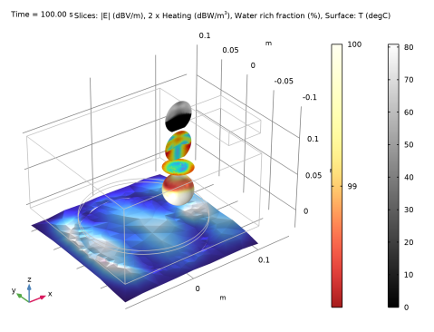
In the Title text area, type Slices: |E| (dBV/m), 2 x Heating (dBW/m<sup>3</sup>), Water rich fraction (%), Surface: T (degC).
7
In the Parameter indicator text field, type Time = eval(t) s.
8
Locate the Plot Settings section. Clear the Plot dataset edges checkbox.
Slice 1
1
Right-click Combined Plot and choose Slice.
2
In the Settings window for Slice, locate the Expression section.
3
In the Expression text field, type 20*log10(emw.normE+1e3).
4
Locate the Plane Data section. From the Plane list, choose xy-planes.
5
In the Planes text field, type 1.
6
Select the Interactive checkbox.
7
In the Shift text field, type -0.05.
8
Locate the Coloring and Style section. From the Color table list, choose Wave.
9
Clear the Color legend checkbox.
Selection 1
1
Right-click Slice 1 and choose Selection.
2
Deformation 1
1
In the Model Builder window, right-click Slice 1 and choose Deformation.
2
In the Settings window for Deformation, locate the Expression section.
3
In the x-component text field, type 0.
4
In the y-component text field, type 0.
5
In the z-component text field, type 20*log10(emw.normE+1e3)-110.
6
Locate the Scale section.
7
Select the Scale factor checkbox. In the associated text field, type 5E-4.
Surface 1
1
In the Model Builder window, right-click Combined Plot and choose Surface.
2
In the Settings window for Surface, locate the Expression section.
3
In the Expression text field, type min(T,100[degC]).
4
From the Unit list, choose °C.
5
Locate the Coloring and Style section. From the Color table list, choose ThermalLight.
Selection 1
1
Right-click Surface 1 and choose Selection.
2
In the Settings window for Selection, locate the Selection section.
3
Click  Paste Selection.
4
In the Paste Selection dialog, type 32-35, 37-40 in the Selection text field.
5
Line 1
1
In the Model Builder window, right-click Combined Plot and choose Line.
2
In the Settings window for Line, locate the Expression section.
3
In the Expression text field, type 1.
4
Locate the Coloring and Style section. From the Coloring list, choose Uniform.
5
From the Color list, choose Gray.
Selection 1
1
Right-click Line 1 and choose Selection.
2
In the Settings window for Selection, locate the Selection section.
3
Click  Paste Selection.
4
In the Paste Selection dialog, type 1-8, 10, 11, 13, 14, 18, 20, 23, 25, 29-45, 47, 48, 50, 51, 55, 57, 60, 62 in the Selection text field.
5
Slice 2
1
In the Model Builder window, right-click Combined Plot and choose Slice.
2
In the Settings window for Slice, locate the Expression section.
3
In the Expression text field, type log10(emw.Qh).
4
Locate the Plane Data section. From the Plane list, choose xy-planes.
5
In the Planes text field, type 1.
6
Locate the Coloring and Style section. From the Color table list, choose Prism.
7
Clear the Color legend checkbox.
Selection 1
1
Right-click Slice 2 and choose Selection.
2
Transformation 1
1
In the Model Builder window, right-click Slice 2 and choose Transformation.
2
In the Settings window for Transformation, locate the Transformation section.
3
In the z text field, type 0.03.
Slice 3
1
Right-click Slice 2 and choose Duplicate.
2
In the Model Builder window, click Slice 3.
3
In the Settings window for Slice, locate the Plane Data section.
4
From the Plane list, choose zx-planes.
5
In the Planes text field, type 1.
6
Locate the Inherit Style section. From the Plot list, choose Slice 2.
Transformation 1
1
In the Model Builder window, click Transformation 1.
2
In the Settings window for Transformation, locate the Transformation section.
3
In the z text field, type 0.06.
Slice 4
1
In the Model Builder window, under Results > Combined Plot right-click Slice 2 and choose Duplicate.
2
In the Settings window for Slice, locate the Expression section.
3
In the Expression text field, type ht.theta1.
4
From the Unit list, choose %.
5
Locate the Plane Data section. From the Plane list, choose zx-planes.
6
In the Planes text field, type 1.
7
Locate the Coloring and Style section. From the Color table list, choose GrayScale.
8
Select the Color legend checkbox.
Transformation 1
1
In the Model Builder window, expand the Slice 4 node, then click Transformation 1.
2
In the Settings window for Transformation, locate the Transformation section.
3
In the z text field, type 0.1.
4
Clear the Apply to dataset edges checkbox.