PDF

Fast Asymptotic Radar Cross-Section Analysis of a Conductive Sphere
Introduction
This example uses asymptotic techniques to study the radar cross-section (RCS) response of a conductive sphere. The selected physics interface transforms the incident plane-wave field on the boundaries to the far-field using the Stratton–Chu formula. The computed results are compared to the well-known asymptotic RCS value of a conductive sphere in the optical region. The optical region is one of three scattering regions used in radar terminology. The other regions are the Rayleigh and Mie regions. See Table 1 below for a discussion of the characteristic sphere size a for the three scattering regions.
r0 << λ0
r0 >> λ0, conventionally 2πr0/λ0 > 10
Figure 1: The background field incident on the surface of a PEC sphere is plotted with the 3D RCS pattern that is partially transparent.
Model Definition
The Electromagnetic Waves, Asymptotic Scattering physics interface is useful when approximating the scattered far-field of an object configured only by a perfect electric conductor (PEC) boundary condition. The incident background field is a z-polarized wave propagating along the positive x-axis. Only PEC is available in this physics interface. So, the sphere is set to a PEC by default. The far-field calculation feature transforms the surface background field on the metallic scatterer to the far-field. There is no need to add a surrounding air domain and absorbing boundary condition as in a typical finite element analysis.
Results and Discussion
After computation, two default plots are generated. They are the surface plot of the background field on the sphere (Figure 2) and the 1D plot of the RCS (Figure 3). Figure 2 shows the z-component of the background field projected on the conductive sphere. The field has a sinusoidal spatial variation with a wavelength corresponding to the simulation frequency 30 GHz.
Figure 2: The z-component of the background electric field on the surface of a metallic sphere modeled as perfect electric conductor.
The default RCS plot is modified to show the logarithmic value of the bistatic RCS. When calculating the monostatic RCS, the incident angle of the background field increases corresponding to every RCS observation angle. Here, the bistatic analysis is simpler: the propagation direction of the background field is fixed at one angle while measuring the RCS at each angle of observation. For an electrically large sphere in the optical region, the reference RCS value can be calculated by
where r0 is the radius of a sphere.
Figure 3: The dB-scaled bistatic RCS plot with the known asymptotic RCS value of the sphere in the optical region.
Notes About the COMSOL Implementation
The Compute action does not perform a real computation. Instead, it is a preprocess for the far-field transformation used in the results plot. At the moment you click one of the generated default plots, the postprocessing of a far-field expression is conducted. Though it is a fast asymptotic method, it still takes time to visualize the 3D far-field response of a finely meshed structure, which is an electrically large scatterer in terms of wavelengths.
The usage of this specific physics interface is limited to a convex-shaped scatterer where multiple reflections are not expected.
Application Library path: RF_Module/Scattering_and_RCS/rcs_sphere_asymptotic
Modeling Instructions
From the File menu, choose New.
New
In the New window, click  Model Wizard.
Model Wizard
1
In the Model Wizard window, click  3D.
2
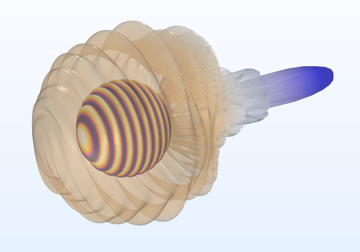
In the Select Physics tree, select Radio Frequency > Electromagnetic Waves, Asymptotic Scattering (ewas).
3
Click Add.
4
Click  Study.
5
In the Select Study tree, select General Studies > Frequency Domain.
6
Global Definitions
Parameters 1
1
In the Model Builder window, under Global Definitions click Parameters 1.
2
In the Settings window for Parameters, locate the Parameters section.
3
Study 1
Step 1: Frequency Domain
Define the study frequency ahead of performing any frequency-dependent operation such as building mesh. The physics-controlled mesh uses the specified frequency value.
1
In the Model Builder window, under Study 1 click Step 1: Frequency Domain.
2
In the Settings window for Frequency Domain, locate the Study Settings section.
3
In the Frequencies text field, type f0.
Geometry 1
Sphere 1 (sph1)
1
In the Geometry toolbar, click  Sphere.
2
In the Settings window for Sphere, locate the Size section.
3
In the Radius text field, type r0.
4
Click  Build All Objects.
Electromagnetic Waves, Asymptotic Scattering (ewas)
Use the default settings. The z-polarized plane-wave background field is propagating in the positive x direction in vacuum.
Mesh 1
In the Model Builder window, under Component 1 (comp1) right-click Mesh 1 and choose Build All.
Study 1
In the Study toolbar, click  Compute.
Results
Background Electric Field (ewas)
This is the background electric field (z-component) illuminating the sphere.
RCS, xy-plane
1
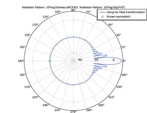
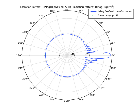
In the Model Builder window, expand the Results > Radar Cross Section (ewas) node, then click Radiation Pattern 1.
2
In the Settings window for Radiation Pattern, type RCS, xy-plane in the Label text field.
3
Locate the Evaluation section. Find the Angles subsection. In the Number of angles text field, type 720.
4
Click to expand the Legends section. Select the Show legends checkbox.
5
From the Legends list, choose Manual.
6
RCS, known asymptotic in the optical region
1
Right-click RCS, xy-plane and choose Duplicate.
2
In the Settings window for Radiation Pattern, type RCS, known asymptotic in the optical region in the Label text field.
3
Locate the Expression section. In the Expression text field, type 10*log10(pi*r0^2).
4
Locate the Legends section. In the table, enter the following settings:
5
Click to expand the Coloring and Style section. Find the Line style subsection. From the Line list, choose None.
6
Find the Line markers subsection. From the Marker list, choose Circle.
7
In the Number text field, type 1.
Radar Cross Section (ewas)
1
In the Model Builder window, click Radar Cross Section (ewas).
2
In the Settings window for Polar Plot Group, locate the Axis section.
3
Select the Manual axis limits checkbox.
4
In the r minimum text field, type -50.
5
In the Radar Cross Section (ewas) toolbar, click  Plot.
The computed bistatic radar cross-section (RCS) results are compared to the known asymptotic backward scattering RCS value in the optical region.