|
|
|

|
1
|
|
2
|
|
3
|
Click Add.
|
|
4
|
Click
|
|
5
|
|
6
|
Click
|
|
1
|
|
2
|
|
3
|
|
4
|
|
5
|
Click to expand the Layers section. In the table, enter the following settings:
|
|
1
|
|
2
|
|
3
|
|
4
|
|
5
|
|
6
|
|
7
|
|
8
|
|
1
|
|
2
|
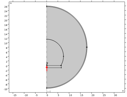
Select the object c1 only.
|
|
3
|
|
4
|
|
5
|
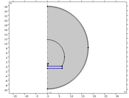
Select the object r1 only.
|
|
6
|
Click
|
|
1
|
|
2
|
|
3
|
|
4
|
|
5
|
|
1
|
|
2
|
|
3
|
|
4
|
|
5
|
Locate the Layers section. In the table, enter the following settings:
|
|
1
|
|
2
|
|
3
|
|
4
|
|
5
|
|
6
|
|
7
|
|
8
|
Click
|
|
1
|
|
2
|
|
3
|
|
4
|
|
5
|
|
6
|
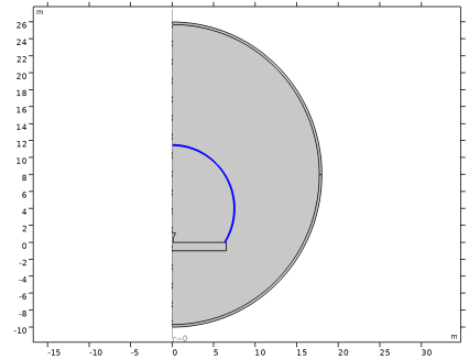
Select the object r3 only.
|
|
7
|
Click
|
|
8
|
|
1
|
|
2
|
|
1
|
|
2
|
|
3
|
|
4
|
|
5
|
|
1
|
|
1
|
In the Model Builder window, under Component 1 (comp1) click Electromagnetic Waves, Frequency Domain (emw).
|
|
2
|
In the Settings window for Electromagnetic Waves, Frequency Domain, click to expand the Discretization section.
|
|
3
|
|
4
|
|
1
|
|
3
|
|
4
|
|
5
|
Clear the Enable active port feedback checkbox.
|
|
6
|
Select the Activate slit condition on interior port checkbox.
|
|
7
|
Click Toggle Power Flow Direction.
|
|
1
|
|
1
|
|
3
|
|
4
|
|
1
|
|
3
|
In the Settings window for Transition Boundary Condition, locate the Transition Boundary Condition section.
|
|
4
|
|
5
|
|
6
|
|
7
|
|
1
|
Go to the Add Material window.
|
|
2
|
|
3
|
Click the Add to Component button in the window toolbar.
|
|
4
|
|
1
|
|
2
|
|
3
|
|
5
|
Locate the Material Contents section. In the table, enter the following settings:
|
|
1
|
|
1
|
|
2
|
|
3
|
|
1
|
|
2
|
|
3
|
|
4
|
|
5
|
|
6
|
|
7
|
Click to expand the Range section. Locate the Coloring and Style section. From the Color table list, choose Ranitomeya.
|
|
8
|
|
1
|
|
2
|
|
3
|
|
4
|
|
5
|
Clear the Color legend checkbox.
|
|
6
|
|
1
|
|
3
|
|
1
|
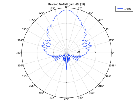
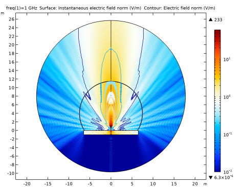
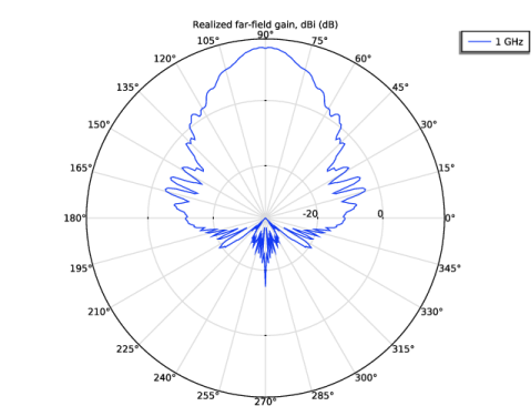
In the Model Builder window, expand the Results > 2D Far Field (emw) node, then click Radiation Pattern 1.
|
|
2
|
|
3
|
|
4
|
Locate the Evaluation section. Find the Angles subsection. In the Number of angles text field, type 360.
|
|
5
|
|
6
|
|
7
|
|
8
|
|
1
|
|
2
|
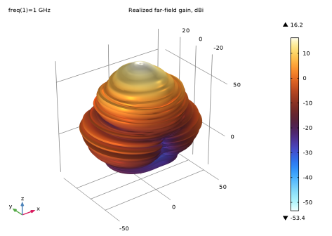
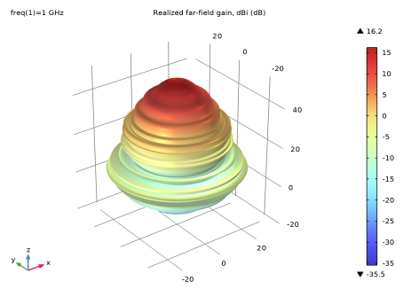
In the Settings window for 3D Plot Group, type 3D Far Field, Gain (emw), TE11 in the Label text field.
|
|
1
|
In the Model Builder window, expand the 3D Far Field, Gain (emw), TE11 node, then click Radiation Pattern 1.
|
|
2
|
|
3
|
|
4
|
Locate the Evaluation section. Find the Angles subsection. In the Azimuthal angle variable text field, type angle.
|
|
5
|
|
1
|
|
2
|
|
1
|
|
2
|
|
3
|
|
1
|
|
2
|
|
1
|
|
2
|
|
3
|
Click
|
|
1
|
|
2
|
|
3
|
|
4
|
|
1
|
|
2
|
|
3
|
|
1
|
|
2
|
|
3
|
|
4
|
|
5
|
|
1
|
|
2
|
|
3
|
|
4
|
|
5
|
|
1
|
|
2
|
|
3
|
|
4
|
|
1
|
|
2
|
|
3
|
|
4
|
|
1
|
|
2
|
|
3
|
|
4
|
|
1
|
|
2
|
|
3
|
|
4
|
|
1
|
|
2
|
|
3
|
Clear the Plot dataset edges checkbox.
|
|
4
|
|
5
|