|
|
|
|
1
|
|
2
|
|
3
|
Click Add.
|
|
4
|
Click
|
|
5
|
|
6
|
Click
|
|
1
|
|
2
|
|
3
|
|
1
|
|
2
|
|
1
|
|
2
|
Browse to the model’s Application Libraries folder and double-click the file mri_coil_geom_sequence.mph.
|
|
3
|
|
4
|
|
5
|
|
1
|
|
2
|
|
3
|
Click
|
|
4
|
|
1
|
|
2
|
|
3
|
|
4
|
|
5
|
|
6
|
Click
|
|
1
|
|
2
|
|
3
|
|
4
|
|
5
|
Click
|
|
6
|
In the Paste Selection dialog, type 9 10 11 12 14 16 19 21 31 33 36 38 66 67 76 77 85 87 90 92 95 97 100 102 in the Selection text field.
|
|
7
|
|
1
|
|
2
|
|
3
|
|
5
|
|
1
|
|
2
|
|
3
|
|
5
|
|
1
|
|
2
|
|
3
|
|
4
|
|
1
|
|
2
|
|
3
|
|
4
|
|
1
|
|
2
|
|
1
|
|
2
|
|
3
|
|
4
|
Click
|
|
5
|
|
6
|
Click OK.
|
|
1
|
In the Model Builder window, under Component 1 (comp1) right-click Materials and choose Blank Material.
|
|
2
|
|
1
|
|
2
|
|
3
|
|
1
|
|
1
|
|
2
|
|
4
|
|
5
|
|
1
|
|
3
|
|
4
|
|
5
|
|
6
|
|
1
|
|
3
|
|
4
|
|
5
|
|
6
|
Click the Split by Connectivity button in the window toolbar.
|
|
1
|
|
2
|
|
3
|
|
1
|
|
2
|
|
3
|
|
4
|
Click
|
|
1
|
|
2
|
|
3
|
Click
|
|
5
|
Click
|
|
6
|
|
7
|
|
8
|
|
9
|
Click Replace.
|
|
10
|
|
1
|
In the Model Builder window, expand the Results > Datasets node, then click Study 1/Solution 1 (sol1).
|
|
1
|
|
2
|
|
3
|
|
1
|
|
2
|
|
3
|
|
1
|
|
2
|
|
3
|
|
4
|
|
5
|
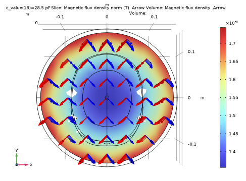
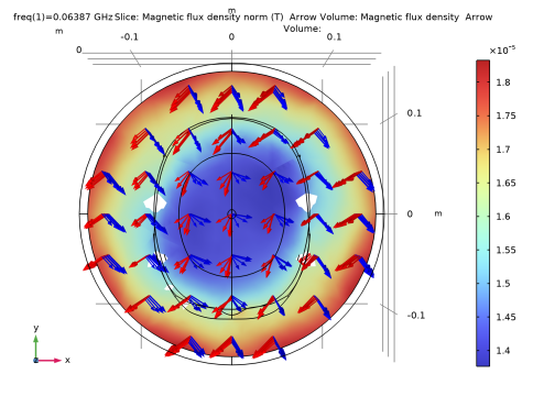
Click Replace Expression in the upper-right corner of the Expression section. From the menu, choose Component 1 (comp1) > Electromagnetic Waves, Frequency Domain > Magnetic > emw.normB - Magnetic flux density norm - T.
|
|
1
|
|
2
|
In the Settings window for Arrow Volume, click Replace Expression in the upper-right corner of the Expression section. From the menu, choose Component 1 (comp1) > Electromagnetic Waves, Frequency Domain > Magnetic > emw.Bx,...,emw.Bz - Magnetic flux density.
|
|
1
|
|
2
|
|
3
|
|
4
|
|
5
|
|
6
|
|
7
|
|
8
|
|
9
|
|
1
|
|
2
|
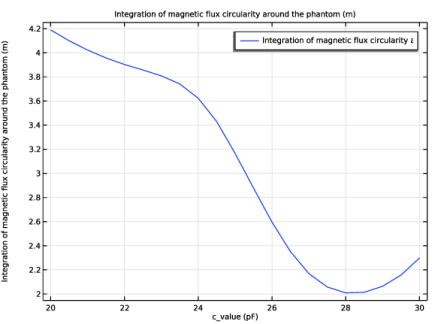
In the Settings window for Global, click Replace Expression in the upper-right corner of the y-Axis Data section. From the menu, choose Component 1 (comp1) > Definitions > Variables > intBaxialratiodB - Integration of magnetic flux circularity around the phantom - m.
|
|
1
|
|
2
|
|
1
|
|
2
|
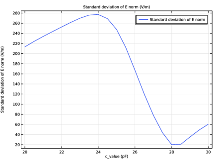
In the Settings window for Global, click Replace Expression in the upper-right corner of the y-Axis Data section. From the menu, choose Component 1 (comp1) > Definitions > Variables > stdev - Standard deviation of E norm - V/m.
|
|
1
|
|
2
|
|
1
|
|
2
|
|
1
|
In the Model Builder window, under Component 1 (comp1) right-click Materials and choose Blank Material.
|
|
3
|
|
1
|
|
2
|
Go to the Add Study window.
|
|
3
|
|
4
|
Click the Add Study button in the window toolbar.
|
|
5
|
|
1
|
|
2
|
|
3
|
|
1
|
|
2
|
|
3
|
|
1
|
|
2
|
|
1
|
|
2
|
In the Settings window for Slice, click Replace Expression in the upper-right corner of the Expression section. From the menu, choose Component 1 (comp1) > Electromagnetic Waves, Frequency Domain > Magnetic > emw.normB - Magnetic flux density norm - T.
|
|
3
|
|
4
|
|
1
|
|
2
|
In the Settings window for Arrow Volume, click Replace Expression in the upper-right corner of the Expression section. From the menu, choose Component 1 (comp1) > Electromagnetic Waves, Frequency Domain > Magnetic > emw.Bx,...,emw.Bz - Magnetic flux density.
|
|
1
|
|
2
|
|
3
|
|
4
|
|
5
|
|
6
|
|
1
|
|
2
|
|
1
|
|
2
|
|
3
|
|
4
|
Click Replace Expression in the upper-right corner of the Expressions section. From the menu, choose Component 1 (comp1) > Definitions > Variables > intBaxialratiodB - Integration of magnetic flux circularity around the phantom - m.
|
|
5
|
Click
|
|
1
|
|
2
|
|
3
|
|
4
|
Click Replace Expression in the upper-right corner of the Expressions section. From the menu, choose Component 1 (comp1) > Definitions > Variables > stdev - Standard deviation of E norm - V/m.
|
|
5
|
Click
|
|
1
|
|
2
|
Click
|
|
1
|
|
2
|
|
3
|
Click
|
|
4
|
Browse to the model’s Application Libraries folder and double-click the file mri_coil_parameters.txt.
|
|
1
|
|
2
|
|
3
|
|
4
|
|
5
|
|
6
|
Click to expand the Layers section. In the table, enter the following settings:
|
|
7
|
Clear the Layers on side checkbox.
|
|
8
|
Select the Layers on bottom checkbox.
|
|
9
|
Select the Layers on top checkbox.
|
|
1
|
|
2
|
|
3
|
|
4
|
Click
|
|
1
|
|
2
|
|
3
|
|
4
|
|
5
|
|
1
|
|
2
|
Select the object c1 only.
|
|
3
|
|
1
|
|
2
|
|
3
|
|
4
|
|
5
|
|
6
|
On the object ccur1, select Boundaries 2 and 3 only.
|
|
1
|
|
2
|
|
3
|
|
4
|
Locate the Distances section. In the table, enter the following settings:
|
|
1
|
|
2
|
|
1
|
|
2
|
Select the object ext2 only.
|
|
3
|
|
4
|
|
1
|
|
2
|
|
3
|
|
4
|
|
5
|
|
1
|
|
2
|
Click in the Graphics window and then press Ctrl+A to select all objects.
|
|
3
|
|
1
|
|
2
|
|
3
|
|
4
|
|
5
|
On the object csur1, select Boundaries 3–6, 9, 10, 21, 22, 33, 34, 36, 39, 51, 52, 63, and 64 only.
|
|
1
|
|
2
|
|
3
|
|
4
|
|
5
|
|
6
|
Locate the Layers section. In the table, enter the following settings:
|
|
7
|
Clear the Layers on side checkbox.
|
|
8
|
Select the Layers on top checkbox.
|
|
1
|
|
2
|
|
3
|
|
4
|
|
5
|
|
1
|
|
2
|
|
3
|
|
4
|