PDF

Microstrip Patch Antenna Surrogate Model
Introduction
This example builds surrogate models with deep neural network (DNN) training to quickly estimate the performance of a microstrip patch antenna based on four design parameters: patch length, tuning stub length, dielectric constant of a substrate, and frequency. The model also simulates a full finite element (FEM) model using asymptotic waveform evaluation of the computed S-parameters to efficiently evaluate the frequency response with fine frequency resolution. This approach can be much faster than a conventional discrete frequency sweep, which may take a long time due to the large number of samples. The full model is used to verify the accuracy of the surrogate models.
Figure 1: Base microstrip patch antenna model with four parameters, used for generating surrogate models.
Model Definition
The embedded model is based on the Microstrip Patch Antenna model from the RF Module Application Library. It includes:
Study for Training Data Generation
To efficiently generate the input parameter space and the output quantities of interest, two geometry sampling features are added separately under the Definitions. One is for the antenna’s realized gain configured based on the far-field calculation boundary feature selections. The other is for near field, sampling the norm of the electric field on the top surface of the antenna substrate.
The number of input point is set to 1000. The Surrogate Modeling study step is executed in combination with a Frequency Domain study step.
Deep Neural Network (DNN) Training
DNN training for each quantity of interest is performed with separate layer configurations and training settings.
Table 3: DNN Settings.
Learning rate, weight decay, and batch size were tuned to minimize the validation loss with the given training data and preventing overfitting.
Study for Full FEM model
The output from the DNN-trained surrogate model can be visualized by comparing it to results from the full FEM model. Adaptive Frequency Sweep, based on asymptotic waveform evaluation with computed S-parameters, is used to achieve S-parameter and other quantities of interest with a finer frequency resolution, 0.5 MHz. To reduce the file size, only the solutions on the far-field calculation boundaries and the top surface of the substrate were saved.
Results and Discussion
The following analyses are addressed between the full model and DNN-trained surrogated models:
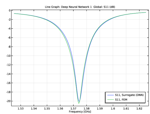
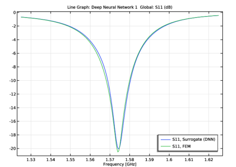
S-parameter (S11) in dB comparison.
The DNN-trained surrogate models can predict quantities of interest such as S-parameters, near- and far-field intensities, almost instantly, while producing results that closely resembles those of full models. Minor discrepancies are anticipated to diminish with improved DNN configuration.
Figure 2: Comparison of S-parameters between the full model and the DNN-trained surrogate model.
Figure 3: Norm of the electric field on the top surface of the antenna for the full model (right) and the DNN-trained surrogated model (left).
Figure 4: Realized far-field gain for the full model (right) and the DNN-trained surrogate model (left).
Notes About the Implementation
The size of the data generated for surrogate model training and the DNN configurations may be subjected to change in order to improve the regression models and enhance accuracy. The specific numbers used in this app are merely examples and maybe adjusted, which could affect the output of the surrogate models.
Application Library path: RF_Module/Antenna_Arrays/microstrip_patch_antenna_surrogate
Modeling Instructions
Application Libraries
1
From the File menu, choose Application Libraries.
2
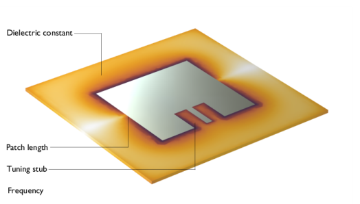
In the Application Libraries window, select RF Module > Antenna Arrays > microstrip_patch_antenna_inset in the tree.
3
Global Definitions
Parameters 1
1
In the Model Builder window, under Global Definitions click Parameters 1.
2
In the Settings window for Parameters, locate the Parameters section.
3
Several parameters have been introduced for deep neural network training. The parameters l_patch, l_stub, e_r, and f0 will be used as input parameters for generating surrogate model training data.
Component 1 (comp1)
In the Model Builder window, expand the Component 1 (comp1) node.
Materials
Substrate (mat2)
1
In the Model Builder window, expand the Component 1 (comp1) > Materials node, then click Substrate (mat2).
2
In the Settings window for Material, locate the Material Contents section.
3
Electromagnetic Waves, Frequency Domain (emw)
In the Model Builder window, expand the Component 1 (comp1) > Electromagnetic Waves, Frequency Domain (emw) node.
Far-Field Calculation 1
1
In the Model Builder window, expand the Component 1 (comp1) > Electromagnetic Waves, Frequency Domain (emw) > Far-Field Domain 1 node, then click Far-Field Calculation 1.
2
In the Settings window for Far-Field Calculation, locate the Boundary Selection section.
3
Click  Create Selection.
4
In the Create Selection dialog, type Far-Field Calculation in the Selection name text field.
5
The explicit selection created directly from the Far-Field Calculation feature assists in configuring the geometry sampling area for generating training data.
Definitions
Geometry Sampling, Far-Field Calculation
1
In the Definitions toolbar, click  Geometry Sampling.
2
In the Settings window for Geometry Sampling, type Geometry Sampling, Far-Field Calculation in the Label text field.
3
Locate the Geometric Entity Selection section. From the Geometric entity level list, choose Boundary.
4
From the Selection list, choose Far-Field Calculation.
Surrogate Model Sampling
Geometry Sampling, Substrate
1
In the Definitions toolbar, click  Geometry Sampling.
2
In the Settings window for Geometry Sampling, type Geometry Sampling, Substrate in the Label text field.
3
Locate the Geometric Entity Selection section. From the Geometric entity level list, choose Boundary.
4
The surrogate model training data for deep neural network training is not generated across the entire simulation domain, but only within specific areas of interest. For example, the near-field data, specifically the electric field norm, is sampled and trained on the substrate surface, including the radiating patch area. Far-field values are collected at the boundaries where the near-field to far-field transformation is performed.
In the first study, surrogate model training data is generated for S-parameters, electric field norm, and realized far-field gain. For each variable of interest, data is generated by systematically varying the patch length, impedance-matching stub length, dielectric constant, and operating frequency.
Study 1
Solver Configurations
1
In the Model Builder window, expand the Study 1 node.
2
Right-click Study 1 > Solver Configurations and choose Delete Configurations.
Step 1: Frequency Domain
1
In the Settings window for Frequency Domain, locate the Study Settings section.
2
In the Frequencies text field, type f0.
3
In the Model Builder window, click Study 1.
4
In the Settings window for Study, type Study, Data Generation for Surrogate Model Training in the Label text field.
Surrogate Model Training
1
In the Study toolbar, click  More Study Extensions and choose Surrogate Model Training.
2
In the Settings window for Surrogate Model Training, locate the Quantities of Interest section.
3
4
S-parameter S11dB is a global variable and geometry sampling is not required.
5
6
7
From the Geometry sampling list, choose Geometry Sampling, Substrate.
8
9
10
From the Geometry sampling list, choose Geometry Sampling, Far-Field Calculation.
11
Locate the Input Parameters section. Click  Add.
12
13
In the Lower bound text field, type 50[mm].
14
In the Upper bound text field, type 54[mm].
15
16
17
18
In the Lower bound text field, type 12.5[mm].
19
In the Upper bound text field, type 18.5[mm].
20
21
22
In the Lower bound text field, type 3.13.
23
In the Upper bound text field, type 3.63.
24
25
26
In the Lower bound text field, type freq_min.
27
In the Upper bound text field, type freq_max.
28
In the Unit text field, type Hz.
29
Find the Sampling settings subsection. In the Number of input points text field, type 1000.
 
30
In the Study toolbar, click  Compute.
31
Click  Clear Solutions.
The necessary data for training is generated in the form of tables, and there is no need to retain the solution. By removing the solution, the model file size can be reduced.
Results
2D Far Field (emw), 3D Far Field, Gain (emw), Electric Field (emw), Electric Field, Logarithmic (emw)
1
In the Model Builder window, under Results, Ctrl-click to select Electric Field (emw), Electric Field, Logarithmic (emw), 2D Far Field (emw), and 3D Far Field, Gain (emw).
2
Train each quantity of interest using a deep neural network. Each hidden layer uses the tanh> activation function, except for the last hidden layer for the field quantities, which uses the Sigmoid function to prevent over-truncation of maximum values. The output layer uses a linear activation function to leave the output unmodified.
Global Definitions
Deep Neural Network 1
1
In the Home toolbar, click  Functions and choose Global > Deep Neural Network.
2
In the Settings window for Deep Neural Network, locate the Data section.
3
From the Data source list, choose Result table.
4
Locate the Data Column Settings section. In the table, enter the following settings:
5
6
In the Name text field, type dnn_S11dB.
7
Locate the Layers section. Click  Add Hidden Layer.
8
In the Output features text field, type 256.
9
Click  Add Hidden Layer.
10
In the Output features text field, type 256.
11
Click  Add Hidden Layer.
12
In the Output features text field, type 256.
13
Click  Add Hidden Layer.
14
In the Output features text field, type 128.
15
Click  Add Hidden Layer.
16
In the Output features text field, type 64.
17
Click  Add Hidden Layer.
18
In the Output features text field, type 32.
19
20
From the Activation list, choose Linear (none).
21
Locate the Training, Validation, and Test section. In the Learning rate text field, type 3e-4.
22
In the Weight decay text field, type 2e-4.
23
In the Batch size text field, type 1024.
24
From the Loss function list, choose Mean absolute error.
25
Find the Stop condition subsection. In the Number of epochs text field, type 20000.
26
Find the Validation/test seed settings subsection. In the Random seed text field, type 1e-6.
Tuning parameter values for Learning rate, Weight decay, Batch size, Loss function, Number of epochs, and Randome seed is application-specific and can vary depending on the quantity of interest and the layer configuration. Minor modifications may reduce the risk of overfitting or lead to undesired results. Therefore, tuning should be done gradually and in small increments.
Deep Neural Network 2
1
In the Home toolbar, click  Functions and choose Global > Deep Neural Network.
2
In the Settings window for Deep Neural Network, locate the Data section.
3
From the Data source list, choose Result table.
4
From the Result table list, choose Design Data (QoI2).
5
Locate the Data Column Settings section. In the table, enter the following settings:
Since only the flat surface of the substrate is evaluated and there is no height variation, the spatial coordinate z is not included.
6
7
In the Name text field, type dnn_normE.
8
Locate the Layers section. Click  Add Hidden Layer.
9
In the Output features text field, type 64.
10
Click  Add Hidden Layer.
11
In the Output features text field, type 128.
12
Click  Add Hidden Layer.
13
In the Output features text field, type 128.
14
Click  Add Hidden Layer.
15
In the Output features text field, type 64.
16
Click  Add Hidden Layer.
17
In the Output features text field, type 32.
18
From the Activation list, choose Sigmoid.
19
20
From the Activation list, choose Linear (none).
21
Locate the Training, Validation, and Test section. In the Learning rate text field, type 5e-4.
22
In the Weight decay text field, type 1e-6.
23
From the Loss function list, choose Mean absolute error.
24
Find the Stop condition subsection. In the Number of epochs text field, type 500.
Deep Neural Network 3
1
In the Home toolbar, click  Functions and choose Global > Deep Neural Network.
2
In the Settings window for Deep Neural Network, locate the Data section.
3
From the Data source list, choose Result table.
4
From the Result table list, choose Design Data (QoI3).
5
Locate the Data Column Settings section. In the table, enter the following settings:
6
7
In the Name text field, type dnn_rGaindBEfar.
8
Locate the Layers section. Click  Add Hidden Layer.
9
In the Output features text field, type 32.
10
Click  Add Hidden Layer.
11
In the Output features text field, type 64.
12
Click  Add Hidden Layer.
13
In the Output features text field, type 64.
14
Click  Add Hidden Layer.
15
In the Output features text field, type 32.
16
From the Activation list, choose Sigmoid.
17
18
From the Activation list, choose Linear (none).
19
Locate the Training, Validation, and Test section. In the Learning rate text field, type 2e-4.
20
In the Weight decay text field, type 2e-7.
21
In the Batch size text field, type 1024.
22
From the Loss function list, choose Mean absolute error.
23
Find the Stop condition subsection. In the Number of epochs text field, type 3000.
Deep Neural Network 1 (dnn_S11dB)
1
In the Model Builder window, click Deep Neural Network 1 (dnn_S11dB).
2
In the Settings window for Deep Neural Network, click  Train Model.
While performing deep neural network training, the validation and training losses can be monitored to determine whether the loss values have converged to a desirable level. Once training is complete, the plotted values are volatile and will be overwritten by subsequent training sessions. To preserve the data, activate the Progress window and click the first toolbar button, Copy Convergence Data to Model. This will generate a table containing up to the last 20,000 epochs. When the Deep neural network training Table window is active, click the Table Graph toolbar button to generate the loss plot.
Deep Neural Network 2 (dnn_normE)
1
In the Model Builder window, click Deep Neural Network 2 (dnn_normE).
2
In the Settings window for Deep Neural Network, click  Train Model.
3
In the Convergence Plot 1 window, click the x-Axis Log Scale button in the window toolbar.
Deep Neural Network 3 (dnn_rGaindBEfar)
1
In the Model Builder window, click Deep Neural Network 3 (dnn_rGaindBEfar).
2
In the Settings window for Deep Neural Network, click  Train Model.
3
In the Convergence Plot 1 window, click the x-Axis Log Scale button in the window toolbar.
The results from the surrogate models will be verified using a full finite element method (FEM) simulation with an adaptive frequency sweep study. This study uses a very fine frequency resolution, which leads to a large model file. Therefore, only the solution on the boundary selection of interest is stored by using the Store in Output option.
Definitions
FEM Data Storage
1
In the Definitions toolbar, click  Explicit.
2
In the Settings window for Explicit, type FEM Data Storage in the Label text field.
3
Locate the Input Entities section. From the Geometric entity level list, choose Boundary.
4
Click  Paste Selection.
5
In the Paste Selection dialog, type 9-12, 16, 21, 26, 32, 33, 37, 40 in the Selection text field.
6
Study, Full Model
1
In the Model Builder window, click Study 2.
2
In the Settings window for Study, type Study, Full Model in the Label text field.
Step 1: Adaptive Frequency Sweep
1
In the Model Builder window, under Study, Full Model click Step 1: Adaptive Frequency Sweep.
2
In the Settings window for Adaptive Frequency Sweep, locate the Study Settings section.
3
In the Frequencies text field, type range(freq_min,500[kHz],freq_max).
4
Click to expand the Store in Output section. In the table, click to select the cell at row number 1 and column number 3.
5
In the Selections list box, select Lumped Port.
6
Under Selections, click  Delete.
7
Under Selections, click  Add.
8
In the Add dialog, select FEM Data Storage in the Selections list.
9
Solver Configurations
1
In the Model Builder window, under Study, Full Model right-click Solver Configurations and choose Delete Configurations.
2
In the Home toolbar, click  Compute.
Functions, including the output of a deep neural network, can be mapped to a Grid dataset for visualization. Use a Grid 1D dataset to plot the regression model of the S-parameters. For field quantities, use a Parametric Surface based on a Grid 3D dataset.
Results
Grid 1D for DNN S-parameter Plot
1
In the Results toolbar, click  More Datasets and choose Grid > Grid 1D.
2
In the Settings window for Grid 1D, type Grid 1D for DNN S-parameter Plot in the Label text field.
3
Locate the Parameter Bounds section. In the Minimum text field, type 1.525.
4
In the Maximum text field, type 1.625.
5
Locate the Data section. From the Source list, choose Function.
6
From the Function list, choose Deep Neural Network 1 (dnn_S11dB).
7
Click to expand the Grid section. Click to expand the Advanced section. Locate the Grid section. In the Resolution text field, type 401.
Grid 3D for DNN Near Field on Substrate
1
In the Results toolbar, click  More Datasets and choose Grid > Grid 3D.
2
In the Settings window for Grid 3D, type Grid 3D for DNN Near Field on Substrate in the Label text field.
3
Locate the Data section. From the Source list, choose Function.
4
From the Function list, choose Deep Neural Network 2 (dnn_normE).
5
Locate the Parameter Bounds section. Find the First parameter subsection. In the Minimum text field, type -0.8*l_sub/1e-3.
6
In the Maximum text field, type 0.8*l_sub/1e-3.
7
Find the Second parameter subsection. In the Minimum text field, type -0.8*l_sub/1e-3.
8
In the Maximum text field, type 0.8*l_sub/1e-3.
9
Find the Third parameter subsection. In the Minimum text field, type -0.8*l_sub/1e-3.
10
In the Maximum text field, type 0.8*l_sub/1e-3.
11
Click to expand the Grid section. In the x resolution text field, type 201.
12
In the y resolution text field, type 201.
13
In the z resolution text field, type 2.
The factor 1e-3 is for scaling based on the geometry unit of millimeters (mm) used in the model.
Parametric Surface for DNN Near Field on Substrate
1
In the Results toolbar, click  More Datasets and choose Parametric Surface.
2
In the Settings window for Parametric Surface, type Parametric Surface for DNN Near Field on Substrate in the Label text field.
3
Locate the Data section. From the Dataset list, choose Grid 3D for DNN Near Field on Substrate.
4
Locate the Parameters section. Find the First parameter subsection. In the Minimum text field, type -1.
5
Find the Second parameter subsection. In the Minimum text field, type -1.
6
Locate the Expressions section. In the x text field, type s1*w_sub/2/1e-3.
7
In the y text field, type s2*l_sub/2/1e-3.
8
In the z text field, type d/2/1e-3.
Grid 3D for DNN Far Field
1
In the Model Builder window, right-click Grid 3D for DNN Near Field on Substrate and choose Duplicate.
2
In the Settings window for Grid 3D, type Grid 3D for DNN Far Field in the Label text field.
3
Locate the Data section. From the Function list, choose Deep Neural Network 3 (dnn_rGaindBEfar).
4
Locate the Grid section. In the x resolution text field, type 71.
5
In the y resolution text field, type 71.
6
In the z resolution text field, type 71.
Parametric Surface for Far Field
1
In the Results toolbar, click  More Datasets and choose Parametric Surface.
2
In the Settings window for Parametric Surface, type Parametric Surface for Far Field in the Label text field.
3
Locate the Data section. From the Dataset list, choose Grid 3D for DNN Far Field.
4
Locate the Parameters section. Find the First parameter subsection. In the Maximum text field, type pi*2.
5
Find the Second parameter subsection. In the Maximum text field, type pi.
6
Locate the Expressions section. In the x text field, type 0.8*l_sub*cos(s1)*sin(s2)/1e-3.
7
In the y text field, type 0.8*l_sub*sin(s1)*sin(s2)/1e-3.
8
In the z text field, type 0.8*l_sub*cos(s2)/1e-3.
S-parameters, Surrogate (DNN) vs. FEM
1
In the Results toolbar, click  1D Plot Group.
2
In the Settings window for 1D Plot Group, type S-parameters, Surrogate (DNN) vs. FEM in the Label text field.
3
Locate the Plot Settings section.
4
Select the x-axis label checkbox. In the associated text field, type Frequency [GHz].
5
Locate the Legend section. From the Position list, choose Lower right.
Line Graph 1
1
Right-click S-parameters, Surrogate (DNN) vs. FEM and choose Line Graph.
2
In the Settings window for Line Graph, locate the Data section.
3
From the Dataset list, choose Grid 1D for DNN S-parameter Plot.
4
Locate the y-Axis Data section. In the Expression text field, type dnn_S11dB(l_patch,l_stub,e_r,x[GHz]).
5
Locate the x-Axis Data section. From the Parameter list, choose Expression.
6
In the Expression text field, type (x/1[m])[GHz].
7
From the Unit list, choose GHz.
The expression for the x-Axis Data is modified to plot the surrogate model output alongside the results of the FEM simulation.
8
Click to expand the Legends section. Select the Show legends checkbox.
9
From the Legends list, choose Manual.
10
Global 1
1
In the Model Builder window, right-click S-parameters, Surrogate (DNN) vs. FEM and choose Global.
2
In the Settings window for Global, locate the Data section.
3
From the Dataset list, choose Study, Full Model/Solution 6 (sol6).
4
Locate the y-Axis Data section. In the table, enter the following settings:
5
Click to expand the Legends section. From the Legends list, choose Manual.
6
7
In the S-parameters, Surrogate (DNN) vs. FEM toolbar, click  Plot.
normE, Surrogate (DNN) vs. FEM
1
In the Results toolbar, click  3D Plot Group.
2
In the Settings window for 3D Plot Group, type normE, Surrogate (DNN) vs. FEM in the Label text field.
3
Locate the Plot Settings section. Clear the Plot dataset edges checkbox.
Surface 1
1
Right-click normE, Surrogate (DNN) vs. FEM and choose Surface.
2
In the Settings window for Surface, locate the Data section.
3
From the Dataset list, choose Parametric Surface for DNN Near Field on Substrate.
4
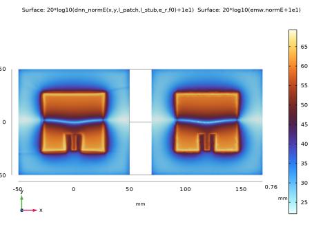
Locate the Expression section. In the Expression text field, type 20*log10(dnn_normE(x,y,l_patch,l_stub,e_r,f0)+1e1).
Adding 1e1 helps produce a more vivid color distribution when plotting on a logarithmic scale.
5
Locate the Coloring and Style section. From the Color table list, choose ThermalWave.
Surface 2
1
In the Model Builder window, right-click normE, Surrogate (DNN) vs. FEM and choose Surface.
2
In the Settings window for Surface, locate the Data section.
3
From the Dataset list, choose Study, Full Model/Solution 6 (sol6).
4
From the Parameter value (freq (GHz)) list, choose 1.575.
5
Locate the Expression section. In the Expression text field, type 20*log10(emw.normE+1e1).
6
Click to expand the Inherit Style section. From the Plot list, choose Surface 1.
Selection 1
1
Right-click Surface 2 and choose Selection.
2
Transformation 1
1
In the Model Builder window, right-click Surface 2 and choose Transformation.
2
In the Settings window for Transformation, locate the Transformation section.
3
In the X text field, type 120.
4
Click the  Go to XY View button in the Graphics toolbar.
5
Click the  Zoom Extents button in the Graphics toolbar.
The output of the function mapped to the Parametric Surface is not compatible with the conventional Radiation Pattern plot. Therefore, a surface plot is used and deformed to create a volumetric 3D radiation pattern shape.
rGaindBEfar, Surrogate (DNN) vs. FEM
1
In the Results toolbar, click  3D Plot Group.
2
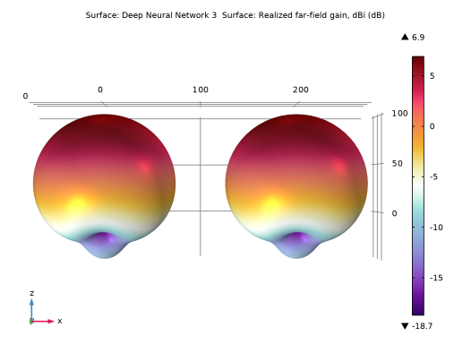
In the Settings window for 3D Plot Group, type rGaindBEfar, Surrogate (DNN) vs. FEM in the Label text field.
3
Locate the Data section. From the Dataset list, choose None.
4
Locate the Color Legend section. Select the Show maximum and minimum values checkbox.
Surface 1
1
Right-click rGaindBEfar, Surrogate (DNN) vs. FEM and choose Surface.
2
In the Settings window for Surface, locate the Data section.
3
From the Dataset list, choose Parametric Surface for Far Field.
4
Locate the Expression section. In the Expression text field, type dnn_rGaindBEfar(x,y,z,l_patch,l_stub,e_r,f0).
5
Locate the Coloring and Style section. From the Color table list, choose Ctenophora.
Deformation 1
1
Right-click Surface 1 and choose Deformation.
2
In the Settings window for Deformation, locate the Expression section.
3
In the x-component text field, type x*(dnn_rGaindBEfar(x,y,z,l_patch,l_stub,e_r,f0))/25.
4
In the y-component text field, type y*(dnn_rGaindBEfar(x,y,z,l_patch,l_stub,e_r,f0))/25.
5
In the z-component text field, type z*(dnn_rGaindBEfar(x,y,z,l_patch,l_stub,e_r,f0))/25.
6
Locate the Scale section.
7
Select the Scale factor checkbox. In the associated text field, type 1.
Surface 2
1
In the Model Builder window, right-click rGaindBEfar, Surrogate (DNN) vs. FEM and choose Surface.
2
In the Settings window for Surface, locate the Data section.
3
From the Dataset list, choose Study, Full Model/Solution 6 (sol6).
4
From the Parameter value (freq (GHz)) list, choose 1.575.
5
Locate the Expression section. In the Expression text field, type emw.rGaindBEfar.
6
Locate the Inherit Style section. From the Plot list, choose Surface 1.
7
Clear the Deform scale factor checkbox.
Selection 1
1
Right-click Surface 2 and choose Selection.
2
In the Settings window for Selection, locate the Selection section.
3
From the Selection list, choose Far-Field Calculation.
Transformation 1
1
In the Model Builder window, right-click Surface 2 and choose Transformation.
2
In the Settings window for Transformation, locate the Transformation section.
3
In the X text field, type 200.
Deformation 1
1
Right-click Surface 2 and choose Deformation.
2
In the Settings window for Deformation, locate the Expression section.
3
In the X-component text field, type x*emw.rGaindBEfar/25.
4
In the Y-component text field, type y*emw.rGaindBEfar/25.
5
In the Z-component text field, type z*emw.rGaindBEfar/25.
6
Locate the Scale section.
7
Select the Scale factor checkbox. In the associated text field, type 1.
8
In the rGaindBEfar, Surrogate (DNN) vs. FEM toolbar, click  Plot.
9
In the Model Builder window, expand the Results > Views node.
Camera
1
In the Model Builder window, expand the Results > Views > View 3D 7 node, then click Camera.
2
In the Settings window for Camera, locate the Camera section.
3
From the View scale list, choose None.
4
Click  Update.
rGaindBEfar, Surrogate (DNN) vs. FEM
1
Click the  Go to XZ View button in the Graphics toolbar.
2
Click the  Zoom Extents button in the Graphics toolbar.
3
In the Model Builder window, under Results click rGaindBEfar, Surrogate (DNN) vs. FEM.