|
|
|
|
1
|
|
2
|
|
1
|
|
2
|
In the Settings window for Study, type Study 2, Quadratic Discretization, AWE in the Label text field.
|
|
3
|
|
1
|
|
2
|
Go to the Add Study window.
|
|
3
|
Find the Studies subsection. In the Select Study tree, select Preset Studies for Selected Physics Interfaces > Frequency Domain, RF Adaptive Mesh.
|
|
4
|
Click the Add Study button in the window toolbar.
|
|
5
|
|
1
|
In the Model Builder window, under Study 3, Linear Discretization for Mesh Adaptation click Step 1: Frequency Domain, RF Adaptive Mesh.
|
|
2
|
|
3
|
Click
|
|
4
|
|
5
|
|
6
|
|
7
|
|
8
|
Click Replace.
|
|
9
|
|
10
|
|
11
|
Clear the Generate default plots checkbox, as the default S-parameter and far-field plots are not of interest for the mesh adaptation study. However, in the following steps a field plot is built, so the mesh adaptation progress can be followed while solving.
|
|
1
|
|
2
|
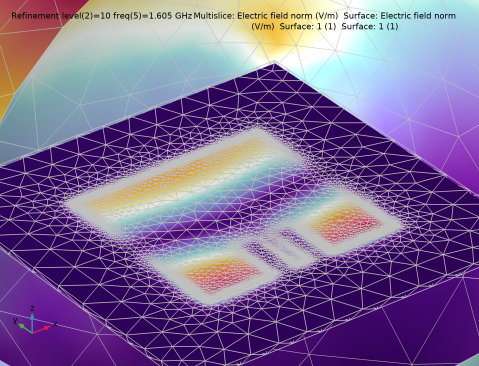
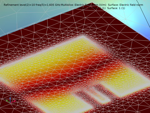
In the Settings window for 3D Plot Group, type Electric Field (emw), Mesh Adaptation in the Label text field.
|
|
3
|
Locate the Data section. From the Dataset list, choose Study 3, Linear Discretization for Mesh Adaptation/Adaptive Mesh Refinement Solutions 1 (sol4).
|
|
4
|
|
1
|
|
2
|
|
3
|
|
4
|
|
5
|
|
1
|
|
2
|
|
3
|
|
1
|
|
2
|
|
3
|
Clear the Show legends checkbox.
|
|
1
|
|
2
|
|
3
|
|
1
|
|
2
|
|
3
|
|
4
|
|
5
|
Click
|
|
1
|
In the Model Builder window, under Results > Electric Field (emw), Mesh Adaptation right-click Surface 1 and choose Duplicate, to add the first of two surface plots to visualize the mesh.
|
|
2
|
|
3
|
|
4
|
|
5
|
|
6
|
Select the Wireframe checkbox.
|
|
1
|
|
2
|
|
3
|
|
1
|
In the Model Builder window, under Study 3, Linear Discretization for Mesh Adaptation click Step 1: Frequency Domain, RF Adaptive Mesh.
|
|
2
|
|
3
|
|
4
|
|
5
|
|
7
|
|
8
|
|
9
|
|
1
|
|
1
|
|
2
|
Go to the Add Study window.
|
|
3
|
Find the Studies subsection. In the Select Study tree, select Preset Studies for Selected Physics Interfaces > Adaptive Frequency Sweep.
|
|
4
|
Click the Add Study button in the window toolbar.
|
|
5
|
|
1
|
In the Settings window for Study, type Study 4, Linear Discretization with Adapted Mesh in the Label text field.
|
|
2
|
Locate the Study Settings section. Clear the Generate default plots checkbox, as we again will not be saving the field in this study. Therefore, there is no point in generating the default field plots.
|
|
1
|
In the Model Builder window, under Study 4, Linear Discretization with Adapted Mesh click Step 1: Adaptive Frequency Sweep.
|
|
2
|
|
3
|
|
4
|
Click to expand the Store in Output section. In the table, enter the following settings:
|
|
6
|
|
7
|
|
8
|
Click OK.
|
|
9
|
|
1
|
|
2
|
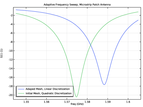
In the Settings window for 1D Plot Group, type S-parameter, Asymptotic Waveform Evaluation on Adapted Mesh in the Label text field.
|
|
3
|
Locate the Data section. From the Dataset list, choose Study 4, Linear Discretization with Adapted Mesh/Solution 16 (sol16).
|
|
4
|
|
5
|
|
6
|
|
1
|
|
2
|
In the Settings window for Global, click Add Expression in the upper-right corner of the y-Axis Data section. From the menu, choose Component 1 (comp1) > Electromagnetic Waves, Frequency Domain > Ports > emw.S11dB - S11 - dB.
|
|
3
|
|
5
|
|
1
|
In the Model Builder window, right-click S-parameter, Asymptotic Waveform Evaluation on Adapted Mesh and choose Paste Global.
|
|
2
|
|
3
|
|
4
|
Locate the Legends section. In the table, enter the following settings:
|
|
5
|