PDF

Parameterized Circulator Geometry
Introduction
This is a template MPH file containing the physics interfaces and the parameterized geometry for the model Impedance Matching of a Lossy Ferrite 3-port Circulator. For a description of that application, see the book Introduction to the RF Module or the documentation for the model Impedance Matching of a Lossy Ferrite 3-Port Circulator.
Application Library path: RF_Module/Ferrimagnetic_Devices/lossy_circulator_3d_geom
Modeling Instructions
From the File menu, choose New.
New
In the New window, click  Model Wizard.
Model Wizard
1
In the Model Wizard window, click  3D.
2
In the Select Physics tree, select Radio Frequency > Electromagnetic Waves, Frequency Domain (emw).
3
Click Add.
4
Click  Study.
5
In the Select Study tree, select General Studies > Frequency Domain.
6
Global Definitions
The geometry is set up using a parameterized approach. This allows you to match the input impedance to that of the connecting waveguide sections by variation of two geometric design parameters.
Parameters 1
1
In the Model Builder window, under Global Definitions click Parameters 1.
2
In the Settings window for Parameters, locate the Parameters section.
3
Here, e_const, me_const, and mu0_const are predefined COMSOL constants for the elementary charge, the electron mass, and the permeability of vacuum, respectfully.
Except for sc_chamfer and sc_ferrite, the other parameters are not used for geometry construction here. However, the physics-based model directly imports this file, and those parameters are included for convenience in later use.
To create the geometry, the 2D cross-section of the circulator is built first. Then, it is extruded into 3D.
Geometry 1
Work Plane 1 (wp1)
1
In the Geometry toolbar, click  Work Plane.
2
In the Settings window for Work Plane, click  Go to Plane Geometry.
Work Plane 1 (wp1) > Plane Geometry
In the Model Builder window, click Plane Geometry.
Start by defining one arm of the circulator and rotate it to build all three arms.
Work Plane 1 (wp1) > Rectangle 1 (r1)
1
In the Work Plane toolbar, click  Rectangle.
2
In the Settings window for Rectangle, locate the Size and Shape section.
3
In the Width text field, type 0.2-0.1/(3*sqrt(3)).
4
In the Height text field, type 0.2/3.
5
Locate the Position section. In the xw text field, type -0.2.
6
In the yw text field, type -0.1/3.
7
Click  Build Selected.
Work Plane 1 (wp1) > Rotate 1 (rot1)
1
In the Work Plane toolbar, click  Transforms and choose Rotate.
2
3
In the Settings window for Rotate, locate the Input section.
4
Select the Keep input objects checkbox.
5
Locate the Rotation section. In the Angle text field, type 120 240.
6
Click  Build Selected.
7
Click the  Zoom Extents button in the Graphics toolbar.
Work Plane 1 (wp1) > Plane Geometry
At this stage, the geometry should appear as shown in the figure below.
1
In the Model Builder window, click Plane Geometry.
Next, build the central connecting region.
Work Plane 1 (wp1) > Circle 1 (c1)
1
In the Work Plane toolbar, click  Circle.
2
In the Settings window for Circle, locate the Size and Shape section.
3
In the Radius text field, type 0.2/(3*sqrt(3)).
4
Click  Build Selected.
Work Plane 1 (wp1) > Difference 1 (dif1)
1
In the Work Plane toolbar, click  Booleans and Partitions and choose Difference.
2
3
In the Settings window for Difference, locate the Difference section.
4
Click to select the  Activate Selection toggle button for Objects to subtract.
5
Select the objects r1, rot1(1), and rot1(2) only.
6
Select the Keep objects to subtract checkbox.
7
Click  Build Selected.
Work Plane 1 (wp1) > Plane Geometry
The constructed geometry is expected to look like the figure presented below.
1
In the Model Builder window, click Plane Geometry.
The remaining of the cross-section is generated using geometric parameters, along with rotation, scaling, and union operations.
Work Plane 1 (wp1) > Rotate 2 (rot2)
1
In the Work Plane toolbar, click  Transforms and choose Rotate.
2
3
In the Settings window for Rotate, locate the Rotation section.
4
In the Angle text field, type 180.
5
Click  Build Selected.
Work Plane 1 (wp1) > Plane Geometry
Apply the scaling for the impedance matching.
Work Plane 1 (wp1) > Scale 1 (sca1)
1
In the Work Plane toolbar, click  Transforms and choose Scale.
2
3
In the Settings window for Scale, locate the Input section.
4
Select the Keep input objects checkbox.
5
Locate the Scale Factor section. In the Factor text field, type sc_chamfer.
6
Click  Build Selected.
Work Plane 1 (wp1) > Union 1 (uni1)
1
In the Work Plane toolbar, click  Booleans and Partitions and choose Union.
2
Select the objects r1, rot1(1), rot1(2), and sca1 only.
3
In the Settings window for Union, locate the Union section.
4
Clear the Keep interior boundaries checkbox.
5
Click  Build Selected.
Work Plane 1 (wp1) > Plane Geometry
After completing these steps, the geometry should match the illustration below.
1
In the Model Builder window, click Plane Geometry.
Apply the scaling for the ferrite region.
Work Plane 1 (wp1) > Scale 2 (sca2)
1
In the Work Plane toolbar, click  Transforms and choose Scale.
2
3
In the Settings window for Scale, locate the Scale Factor section.
4
In the Factor text field, type sc_ferrite.
5
Click  Build Selected.
Work Plane 1 (wp1)
Extruding the 2D cross section into a 3D solid geometry finalizes the geometry definition.
Extrude 1 (ext1)
1
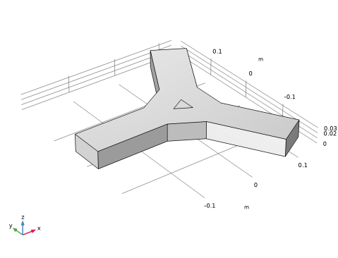
In the Model Builder window, under Component 1 (comp1) > Geometry 1 right-click Work Plane 1 (wp1) and choose Extrude.
2
In the Settings window for Extrude, locate the Distances section.
3
4
Click  Build Selected.
5
Click the  Zoom Extents button in the Graphics toolbar.
Form Union (fin)
1
In the Geometry toolbar, click  Build All.
The resulting geometry is displayed in the following figure.
2
In the Model Builder window, click Form Union (fin).