PDF

Superheated Steam Drying of a Wood Particle
Introduction
Drying of porous media is a crucial process in industries such as food and paper manufacturing. Superheated steam drying (SSD) offers several advantages over other drying methods. For sensitive products like food, SSD helps minimize substance degradation, browning, and oxidation. Additionally, the SSD process can reduce energy consumption by up to 50% and shorten drying time by up to 80% compared to hot-air drying. Superheated steam dryers are typically more compact and require less investment than hot-air dryers. At temperatures above 120°C, SSD also inactivates microorganisms and ensures product hygiene. Despite the high operating temperatures, the degradation rate of product compounds remains relatively low due to the short retention time.
Higher drying rates can be achieved with SSD due to the superior heat transfer properties of superheated steam. It has a higher thermal conductivity and heat capacity than hot air, and it does not resist the diffusion of evaporated moisture in its own vapor. The material to be dried is introduced in the superheated steam flow, where moisture evaporates through convective heating. This heat transfer process is highly effective, as the high heat capacity and thermal conductivity of superheated steam, combined with its low viscosity, facilitate rapid penetration into the material. Consequently, this drying method is particularly effective for porous materials and results in a shorter retention time.
Modeling such processes requires considering multiple physical effects, including fluid flow, heat transfer, and mass transport with evaporation. These effects are strongly coupled, and predefined interfaces in COMSOL Multiphysics can be used to model these phenomena in a hygroscopic porous medium.
This tutorial demonstrates how to model the superheated steam drying process of a spherical wood particle exposed to laminar flow of superheated steam. The evolution of the moisture content on a dry basis within the wood particle is analyzed for different inlet steam temperatures under nonequilibrium conditions. Model parameters are based on those in Ref. 1, where SSD was modeled using an effective diffusivity formulation.
Model Definition
The model solves the coupled heat and mass transfer problem in a domain with a spherical porous wood particle, exposed in laminar flow of a superheated steam. Since the geometry and boundary conditions are symmetrical, only one quarter of the geometry is modeled. Figure 1 depicts the model geometry.
Figure 1: The model geometry.
The computational domain comprises the spherical wood particle, which diameter is equal to 6.2 mm, and a steam flow around the particle. The length of flow domain is 3 cm, height and width are equal to 1 cm.
Heat and moisture transport
The thermodynamic properties of superheated water vapor are described automatically in the Moist Air feature of the Heat Transfer interface. As the input term for water vapor, the relative humidity ϕw from the moisture transport equation is used in the Heat Transfer and Fluid Flow interfaces. To get the properties of the pure vapor we can define the inlet and initial relative humidity values as pa / psat, where pa is an absolute pressure, and psat is the vapor saturation pressure at the inlet temperature.
FLUID FLOW
The Laminar Flow interface solves for compressible Navier–Stokes equations to compute the velocity and pressure fields of the free flow and Brinkman equations to calculate the flow field and pressure distribution of vapor in the porous medium. It is assumed that there is no liquid water in the free flow domain. This means that all the moisture leaves the porous medium under vapor state.
With an additional liquid phase in porous medium capillary effects also arise, and the liquid flow is driven by a pressure gradient and the capillary pressure pc = pg − pl. In this model, the capillary effects are treated by an additional capillary flux term in the transport equation, defined from the capillary pressure gradient by a Darcy’s law:
,
where κ is total permeability of the porous medium, and μl is viscosity of the liquid phase. The capillary pressure pc and relative liquid water permeability κrl are calculated from the van Genuchten model, that is available in the Liquid Water subfeature of Moisture Transport interface.
The liquid-phase velocity is small compared to the vapor velocity. Liquid transport is driven by the gas-phase pressure gradient pg, and its velocity ul is computed with the use of Darcy’s law according to
.
Finally, due to the dimensions of the porous medium, the gravity effects on transport are neglected in both phases.
HEAT TRANSFER
Inside the porous domain, convection of both liquid and gaseous phases contributes to the heat convective term. It is possible to account for the liquid water and vapor phases, by using the liquid saturation calculated by the moisture transport equation.
Averaged heat capacity (ρCp)eff is defined by taking into account the properties of the porous matrix (ρs, Cp,s), vapor (ρg, Cp,g), and liquid water (ρl, Cp,l):
.
For effective thermal conductivity of porous medium keff the user-defined value is used, that was obtained from experiments (Ref. 1).
The combined convection term in the porous media takes the form
.
The capillary flux of enthalpy due to the presence of the liquid water in the pores is included in the following heat source term:
.
The heat of evaporation is inserted as a source term in the heat transfer equation:
,
where Lv (J/mol) is the latent heat of evaporation.
Surface-to-ambient radiation can take significant role under the high steam temperatures. To take it into account, the radiative heat flux is defined on the upside surface of the wood particle:
,
where ε is the surface emissivity, σ is the Stefan–Boltzmann constant, and Tamb is the ambient superheated steam temperature.
Moisture Transport in FREE AND POROUS MEDIUM
Superheated steam drying process implies that equilibrium between liquid and vapor phases cannot be assumed. In this case the liquid saturation and vapor mass fraction are not related, and the water conservation equations for the liquid phase and vapor phase must be solved separately, that is, the nonequilibrium formulation has to be used. See the Heat Transfer Module User’s Guide for the governing equations.
Unlike the equilibrium assumption, the evaporation source is taken into account for the mass conservation equations. The moisture source due to evaporation is calculated as a deviation from the equilibrium state:
,
where Kevap (1/s) is the evaporation rate, pv,eq is the equilibrium vapor pressure, pv is the pressure of water vapor, and R (J/(mol·K) is the universal gas constant.
The equilibrium vapor pressure can be given as a function of water activity aw and vapor saturation pressure psat:
.
The saturation pressure is calculated automatically in the Moist Air feature of Heat Transfer and Moisture Transfer interfaces.
Results
After 1 hour of superheated steam drying, the average moisture content on the dry basis in the wood particle decreases from initial value of 50% to about 5%, when the steam temperature at the inlet is equal to 130°C, and to about 1%, when the inlet temperature is 170°C. We can see almost homogeneous distribution of moisture content in the wood particle at the end of the drying process (Figure 2).
Figure 2: Temperature in the free flow and moisture content in the wood particle after 1 hour of the drying process for inlet steam temperature of 170°C.
As we can see on the Figure 3, the drying process gets faster for increasing values of the inlet temperature.
Figure 3: Average moisture content on dry basis in the wood particle for different values of the inlet temperature.
The nonequilibrium formulation allows us to set inlet temperature much higher then the saturation value, and model different regimes of superheated steam drying.
The Figure 4 shows the average temperature of the wood particle during the drying process.
Figure 4: Average temperature of the wood particle for different values of the inlet temperature.
Reference
1. K.H. Le, N. Hampel, A. Kharaghani, A. Bück, and E. Tsotsas, “Superheated steam drying of single wood particles: A characteristic drying curve model deduced from continuum model simulations and assessed by experiments,” Drying Technology, vol. 36, no. 15, pp. 1866–1881, 2018.
Application Library path: Porous_Media_Flow_Module/Heat_Transfer/superheated_steam_drying
Modeling Instructions
From the File menu, choose New.
New
In the New window, click  Model Wizard.
Model Wizard
1
In the Model Wizard window, click  3D.
2
In the Select Physics tree, select Heat Transfer > Heat and Moisture Transport > Heat and Moisture Flow > Laminar Flow.
3
Click Add.
4
In the Added physics interfaces tree, select Moisture Transport in Air (mt).
5
Click Remove.
6
In the Select Physics tree, select Chemical Species Transport > Moisture Transport > Moisture Transport in Free and Porous Media (mt).
7
Click Add.
8
Click  Study.
9
In the Select Study tree, select General Studies > Time Dependent.
10
Start with specifying the model parameters.
Global Definitions
Parameters 1
1
In the Model Builder window, under Global Definitions click Parameters 1.
2
In the Settings window for Parameters, locate the Parameters section.
3
Now, define the geometry.
Geometry 1
1
In the Model Builder window, under Component 1 (comp1) click Geometry 1.
2
In the Settings window for Geometry, locate the Units section.
3
From the Length unit list, choose cm.
Block 1 (blk1)
1
In the Geometry toolbar, click  Block.
2
In the Settings window for Block, locate the Size and Shape section.
3
In the Width text field, type L.
4
In the Depth text field, type H.
5
In the Height text field, type H.
6
Click  Build Selected.
Sphere 1 (sph1)
1
In the Geometry toolbar, click  Sphere.
2
In the Settings window for Sphere, locate the Size section.
3
In the Radius text field, type dp/2.
4
Locate the Position section. In the x text field, type L/3.
5
In the z text field, type H.
6
Click  Build Selected.
Partition Objects 1 (par1)
1
In the Geometry toolbar, click  Booleans and Partitions and choose Partition Objects.
2
3
In the Settings window for Partition Objects, locate the Partition Objects section.
4
Click to select the  Activate Selection toggle button for Tool objects.
5
6
Select the Keep tool objects checkbox.
7
Click  Build Selected.
Delete Entities 1 (del1)
1
In the Model Builder window, right-click Geometry 1 and choose Delete Entities.
2
In the Settings window for Delete Entities, locate the Entities or Objects to Delete section.
3
From the Geometric entity level list, choose Domain.
4
On the object par1, select Domain 1 only.
5
Click  Build Selected.
Form Union (fin)
In the Geometry toolbar, click  Build All.
Definitions
Define the variable for the moisture content on dry basis.
Variables 1
1
In the Model Builder window, under Component 1 (comp1) right-click Definitions and choose Variables.
2
In the Settings window for Variables, locate the Variables section.
3
Define the water activity as a function of the moisture content on dry basis. The advantage of using functions is that they can be plotted immediately.
Water activity
1
In the Definitions toolbar, click  Analytic.
2
In the Settings window for Analytic, type Water activity in the Label text field.
3
In the Function name text field, type wa.
4
Locate the Definition section. In the Expression text field, type if(X>0.256,1,X/0.256*(2-X/0.256)).
5
In the Arguments text field, type X.
6
Locate the Units section. In the Function text field, type 1.
7
Now, define the selections to simplify the model setup.
Symmetry Boundaries
1
In the Definitions toolbar, click  Explicit.
2
In the Settings window for Explicit, locate the Input Entities section.
3
From the Geometric entity level list, choose Boundary.
4
5
In the Label text field, type Symmetry Boundaries.
Inlet Boundary
1
In the Definitions toolbar, click  Explicit.
2
In the Settings window for Explicit, locate the Input Entities section.
3
From the Geometric entity level list, choose Boundary.
4
5
In the Label text field, type Inlet Boundary.
Outlet Boundary
1
In the Definitions toolbar, click  Explicit.
2
In the Settings window for Explicit, locate the Input Entities section.
3
From the Geometric entity level list, choose Boundary.
4
5
In the Label text field, type Outlet Boundary.
Porous Medium
1
In the Definitions toolbar, click  Explicit.
2
3
In the Settings window for Explicit, type Porous Medium in the Label text field.
Define an average operator in the porous domain, in order to evaluate the average moisture content evolution.
Average 1 (aveop1)
1
In the Definitions toolbar, click  Nonlocal Couplings and choose Average.
2
In the Settings window for Average, locate the Source Selection section.
3
From the Selection list, choose Porous Medium.
Define the ambient conditions that will be used later in the domain and boundary conditions.
Ambient Properties 1 (ampr1)
1
In the Physics toolbar, click  Shared Properties and choose Ambient Properties.
2
In the Settings window for Ambient Properties, locate the Ambient Conditions section.
3
In the Tamb text field, type T_in.
4
In the ϕamb text field, type mt.pA/mt.fpsat(T_in).
Materials
Add porous material to the materials node, but do not define their properties at this point. After setting up the physics interface, COMSOL Multiphysics automatically detects which material properties are needed.
Wood particle
1
In the Model Builder window, under Component 1 (comp1) right-click Materials and choose More Materials > Porous Material.
2
In the Settings window for Porous Material, type Wood particle in the Label text field.
3
Locate the Geometric Entity Selection section. From the Selection list, choose Porous Medium.
4
Click to expand the Appearance section. From the Material type list, choose Wood.
Now, define the domain and boundary conditions for each interface. Start with the Laminar Flow interface, by setting the physical model parameters, initial and boundary conditions, and by adding a Porous Medium domain condition.
Laminar Flow (spf)
1
In the Model Builder window, under Component 1 (comp1) click Laminar Flow (spf).
2
In the Settings window for Laminar Flow, locate the Physical Model section.
3
From the Compressibility list, choose Compressible flow (Ma<0.3).
4
Select the Enable porous media domains checkbox.
Initial Values 1
1
In the Model Builder window, under Component 1 (comp1) > Laminar Flow (spf) click Initial Values 1.
2
In the Settings window for Initial Values, locate the Initial Values section.
3
Specify the u vector as
Wall 1
1
In the Model Builder window, click Wall 1.
2
In the Settings window for Wall, locate the Boundary Condition section.
3
From the Wall condition list, choose Slip.
Inlet 1
1
In the Physics toolbar, click  Boundaries and choose Inlet.
2
In the Settings window for Inlet, locate the Boundary Selection section.
3
From the Selection list, choose Inlet Boundary.
4
Locate the Velocity section. In the U0 text field, type U_in.
Outlet 1
1
In the Physics toolbar, click  Boundaries and choose Outlet.
2
In the Settings window for Outlet, locate the Boundary Selection section.
3
From the Selection list, choose Outlet Boundary.
Symmetry 1
1
In the Physics toolbar, click  Boundaries and choose Symmetry.
2
In the Settings window for Symmetry, locate the Boundary Selection section.
3
From the Selection list, choose Symmetry Boundaries.
Porous Medium 1
1
In the Physics toolbar, click  Domains and choose Porous Medium.
2
In the Settings window for Porous Medium, locate the Domain Selection section.
3
From the Selection list, choose Porous Medium.
Heat Transfer in Moist Air (ht)
Use the ambient temperature defined previously as input for Initial Values.
Initial Values 1
1
In the Model Builder window, under Component 1 (comp1) > Heat Transfer in Moist Air (ht) click Initial Values 1.
2
In the Settings window for Initial Values, locate the Initial Values section.
3
From the T list, choose Ambient temperature (ampr1).
Add another Initial Values node to define the initial temperature of the wood particle equal to 100°C.
Initial Values 2
1
In the Physics toolbar, click  Domains and choose Initial Values.
2
In the Settings window for Initial Values, locate the Domain Selection section.
3
From the Selection list, choose Porous Medium.
4
Locate the Initial Values section. In the T text field, type 100[degC].
Inflow 1
1
In the Physics toolbar, click  Boundaries and choose Inflow.
2
In the Settings window for Inflow, locate the Boundary Selection section.
3
From the Selection list, choose Inlet Boundary.
4
Locate the Upstream Properties section. From the Tustr list, choose Ambient temperature (ampr1).
Outflow 1
1
In the Physics toolbar, click  Boundaries and choose Outflow.
2
In the Settings window for Outflow, locate the Boundary Selection section.
3
From the Selection list, choose Outlet Boundary.
Surface-to-Ambient Radiation 1
1
In the Physics toolbar, click  Boundaries and choose Surface-to-Ambient Radiation.
2
3
In the Settings window for Surface-to-Ambient Radiation, locate the Surface-to-Ambient Radiation section.
4
From the ε list, choose User defined. In the associated text field, type 0.9.
5
From the Tamb list, choose Ambient temperature (ampr1).
Symmetry 1
1
In the Physics toolbar, click  Boundaries and choose Symmetry.
2
In the Settings window for Symmetry, locate the Boundary Selection section.
3
From the Selection list, choose Symmetry Boundaries.
Moist Porous Medium 1
1
In the Physics toolbar, click  Domains and choose Moist Porous Medium.
2
In the Settings window for Moist Porous Medium, locate the Domain Selection section.
3
From the Selection list, choose Porous Medium.
Select the Equivalent thermal conductivity option to specify the user-defined effective thermal conductivity of porous medium.
4
Locate the Porous Medium Model Settings section. From the Effective thermal conductivity list, choose Equivalent thermal conductivity.
Moisture Transport in Free and Porous Media (mt)
Finally, set the domain, initial, and boundary conditions for the Moisture Transport in Free and Porous Medium interface. Switch to Concentrated Species option to model steam flow.
1
In the Model Builder window, under Component 1 (comp1) click Moisture Transport in Free and Porous Media (mt).
2
In the Settings window for Moisture Transport in Free and Porous Media, locate the Physical Model section.
3
From the Mixture type for moist air list, choose Concentrated species.
Hygroscopic Porous Medium 1
1
In the Model Builder window, under Component 1 (comp1) > Moisture Transport in Free and Porous Media (mt) click Hygroscopic Porous Medium 1.
2
Specify water activity function and evaporation rate.
3
In the Settings window for Hygroscopic Porous Medium, locate the Moisture Transport Properties section.
4
In the aw text field, type wa(Xdry).
5
In the Kevap text field, type K0.
Liquid Water 1
1
In the Model Builder window, click Liquid Water 1.
2
In the Settings window for Liquid Water, locate the Liquid Water Properties section.
3
From the Capillary model list, choose Pressure.
Initial Values 1
1
In the Model Builder window, click Initial Values 1.
2
In the Settings window for Initial Values, locate the Initial Values section.
3
In the sl,0 text field, type sl0.
Symmetry 1
1
In the Physics toolbar, click  Boundaries and choose Symmetry.
2
In the Settings window for Symmetry, locate the Boundary Selection section.
3
From the Selection list, choose Symmetry Boundaries.
Initial Values 1
1
In the Model Builder window, under Component 1 (comp1) > Moisture Transport in Free and Porous Media (mt) > Hygroscopic Porous Medium 1 > Moist Air 1 click Initial Values 1.
2
In the Settings window for Initial Values, locate the Initial Values section.
3
In the ϕw,0 text field, type 1.
Symmetry 1
1
In the Physics toolbar, click  Boundaries and choose Symmetry.
2
In the Settings window for Symmetry, locate the Boundary Selection section.
3
From the Selection list, choose Symmetry Boundaries.
Use the ambient temperature and humidity defined previously as input for Initial Values and Inflow.
Initial Values 1
1
In the Model Builder window, under Component 1 (comp1) > Moisture Transport in Free and Porous Media (mt) click Initial Values 1.
2
In the Settings window for Initial Values, locate the Initial Values section.
3
From the ϕw,0 list, choose Ambient relative humidity (ampr1).
Inflow 1
1
In the Physics toolbar, click  Boundaries and choose Inflow.
2
In the Settings window for Inflow, locate the Boundary Selection section.
3
From the Selection list, choose Inlet Boundary.
4
Locate the Upstream Properties section. From the Tustr list, choose Ambient temperature (ampr1).
5
From the ϕw,ustr list, choose Ambient relative humidity (ampr1).
Outflow 1
1
In the Physics toolbar, click  Boundaries and choose Outflow.
2
In the Settings window for Outflow, locate the Boundary Selection section.
3
From the Selection list, choose Outlet Boundary.
Symmetry 1
1
In the Physics toolbar, click  Boundaries and choose Symmetry.
2
In the Settings window for Symmetry, locate the Boundary Selection section.
3
From the Selection list, choose Symmetry Boundaries.
Materials
The porous material properties can now be specified.
Wood particle (pmat1)
1
In the Model Builder window, under Component 1 (comp1) > Materials click Wood particle (pmat1).
2
In the Settings window for Porous Material, locate the Homogenized Properties section.
3
4
Locate the Phase-Specific Properties section. Click  Add Required Phase Nodes.
Solid 1 (pmat1.solid1)
1
In the Model Builder window, click Solid 1 (pmat1.solid1).
2
In the Settings window for Solid, locate the Solid Properties section.
3
In the θs text field, type 1-por.
4
Locate the Material Contents section. In the table, enter the following settings:
Mesh 1
1
In the Model Builder window, under Component 1 (comp1) click Mesh 1.
2
In the Settings window for Mesh, locate the Physics-Controlled Mesh section.
3
From the Element size list, choose Coarse.
4
Click  Build All.
Study 1
The necessary time to dry the product is unknown. An initial guess of 60 minutes is made.
Step 1: Time Dependent
1
In the Model Builder window, under Study 1 click Step 1: Time Dependent.
2
In the Settings window for Time Dependent, locate the Study Settings section.
3
From the Time unit list, choose min.
4
In the Output times text field, type range(0,0.1,1)[s] range(1,10,59)[s] range(1,1,60).
Activate a parametric sweep to run the simulation for different inlet temperature values.
5
Click to expand the Study Extensions section. Select the Auxiliary sweep checkbox.
6
7
8
In the Study toolbar, click  Compute.
To create the plots shown in Figure 2, Figure 3, and Figure 4, reproduce the following steps.
Results
Preferred Units 1
1
In the Results toolbar, click  Configurations and choose Preferred Units.
2
In the Settings window for Preferred Units, locate the Units section.
3
Click  Add Physical Quantity.
4
In the Physical Quantity dialog, select General > Temperature (K) in the tree.
5
6
In the Settings window for Preferred Units, locate the Units section.
7
8
Click  Apply.
Multislice 1
1
In the Model Builder window, expand the Results > Relative Humidity (mt) node, then click Multislice 1.
2
In the Settings window for Multislice, locate the Multiplane Data section.
3
Find the x-planes subsection. In the Planes text field, type 0.
4
Find the y-planes subsection. From the Entry method list, choose Coordinates.
5
In the Coordinates text field, type 0.
6
Find the z-planes subsection. From the Entry method list, choose Coordinates.
7
In the Coordinates text field, type H.
8
In the Relative Humidity (mt) toolbar, click  Plot.
Result Templates
1
In the Results toolbar, click  Result Templates to open the Result Templates window.
2
Go to the Result Templates window.
3
In the tree, select Study 1/Solution 1 (sol1) > Moisture Transport in Free and Porous Media > Saturation (mt).
4
Click the Add Result Template button in the window toolbar.
Results
Multislice 1
1
In the Model Builder window, expand the Saturation (mt) node, then click Multislice 1.
2
In the Settings window for Multislice, locate the Multiplane Data section.
3
Find the x-planes subsection. In the Planes text field, type 0.
4
Find the y-planes subsection. From the Entry method list, choose Coordinates.
5
In the Coordinates text field, type 0.
6
Find the z-planes subsection. From the Entry method list, choose Coordinates.
7
In the Coordinates text field, type H.
8
In the Saturation (mt) toolbar, click  Plot.
Temperature and Moisture Content on Dry Basis
1
In the Results toolbar, click  3D Plot Group.
2
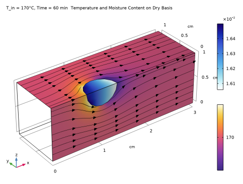
In the Settings window for 3D Plot Group, type Temperature and Moisture Content on Dry Basis in the Label text field.
3
Click to expand the Title section. From the Title type list, choose Manual.
4
In the Title text area, type Temperature and Moisture Content on Dry Basis.
5
In the Parameter indicator text field, type T_in = eval(T_in,°C)°C, Time = eval(t,min) min.
6
Locate the Color Legend section. From the Position list, choose Right double.
Surface 1
1
Right-click Temperature and Moisture Content on Dry Basis and choose Surface.
2
In the Settings window for Surface, locate the Expression section.
3
In the Expression text field, type Xdry.
4
Locate the Coloring and Style section. From the Color table list, choose Kyanite.
Selection 1
1
Right-click Surface 1 and choose Selection.
2
Surface 2
1
In the Model Builder window, right-click Temperature and Moisture Content on Dry Basis and choose Surface.
2
In the Settings window for Surface, locate the Expression section.
3
In the Expression text field, type T.
4
Locate the Coloring and Style section. From the Color table list, choose HeatCameraLight.
Selection 1
1
Right-click Surface 2 and choose Selection.
2
Temperature and Moisture Content on Dry Basis
In the Model Builder window, under Results click Temperature and Moisture Content on Dry Basis.
Streamline Surface 1
1
In the Temperature and Moisture Content on Dry Basis toolbar, click  More Plots and choose Streamline Surface.
2
3
In the Settings window for Streamline Surface, locate the Streamline Positioning section.
4
From the Positioning list, choose Uniform density.
5
Locate the Coloring and Style section. Find the Point style subsection. From the Type list, choose Arrow.
6
From the Color list, choose Black.
7
In the Temperature and Moisture Content on Dry Basis toolbar, click  Plot.
Evaporation Rate
1
In the Home toolbar, click  Add Plot Group and choose 3D Plot Group.
2
In the Settings window for 3D Plot Group, type Evaporation Rate in the Label text field.
3
Click to expand the Selection section. From the Geometric entity level list, choose Domain.
4
From the Selection list, choose Porous Medium.
Surface 1
1
Right-click Evaporation Rate and choose Surface.
2
In the Settings window for Surface, locate the Expression section.
3
In the Expression text field, type mt.G_evap.
4
In the Evaporation Rate toolbar, click  Plot.
Average Moisture Content on Dry Basis
1
In the Results toolbar, click  1D Plot Group.
2
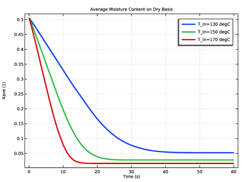
In the Settings window for 1D Plot Group, type Average Moisture Content on Dry Basis in the Label text field.
3
Click to expand the Title section. From the Title type list, choose Manual.
4
In the Title text area, type Average Moisture Content on Dry Basis.
5
Locate the Plot Settings section.
6
Select the x-axis label checkbox. In the associated text field, type Time (s).
7
Select the y-axis label checkbox. In the associated text field, type Xave (1).
Global 1
1
Right-click Average Moisture Content on Dry Basis and choose Global.
2
In the Settings window for Global, locate the y-Axis Data section.
3
4
Click to expand the Coloring and Style section. From the Width list, choose 3.
5
Click to expand the Legends section. Find the Include subsection. Clear the Description checkbox.
6
In the Average Moisture Content on Dry Basis toolbar, click  Plot.
Average Temperature of Wood Particle
1
In the Home toolbar, click  Add Plot Group and choose 1D Plot Group.
2
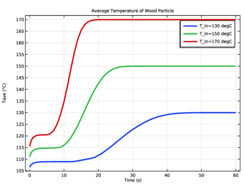
In the Settings window for 1D Plot Group, type Average Temperature of Wood Particle in the Label text field.
3
Locate the Title section. From the Title type list, choose Manual.
4
In the Title text area, type Average Temperature of Wood Particle.
5
Locate the Plot Settings section.
6
Select the x-axis label checkbox. In the associated text field, type Time (s).
7
Select the y-axis label checkbox. In the associated text field, type Tave (°C).
Global 1
1
Right-click Average Temperature of Wood Particle and choose Global.
2
In the Settings window for Global, locate the y-Axis Data section.
3
4
Locate the Coloring and Style section. From the Width list, choose 3.
5
Locate the Legends section. Find the Include subsection. Clear the Description checkbox.
6
In the Average Temperature of Wood Particle toolbar, click  Plot.
Average Relative Humidity
1
In the Results toolbar, click  1D Plot Group.
2
In the Settings window for 1D Plot Group, type Average Relative Humidity in the Label text field.
3
Locate the Title section. From the Title type list, choose Manual.
4
In the Title text area, type Average Relative Humidity.
5
Locate the Plot Settings section.
6
Select the x-axis label checkbox. In the associated text field, type Time (s).
7
Select the y-axis label checkbox. In the associated text field, type phi_ave (1).
Global 1
1
Right-click Average Relative Humidity and choose Global.
2
In the Settings window for Global, locate the y-Axis Data section.
3
4
Locate the Coloring and Style section. From the Width list, choose 3.
5
Locate the Legends section. Find the Include subsection. Clear the Description checkbox.
6
In the Average Relative Humidity toolbar, click  Plot.
Mass Balance
1
In the Results toolbar, click  Evaluation Group.
2
In the Settings window for Evaluation Group, type Mass Balance in the Label text field.
3
Locate the Data section. From the Time selection list, choose Last.
4
Locate the Transformation section. Select the Transpose checkbox.
Global Evaluation 1
1
Right-click Mass Balance and choose Global Evaluation.
2
In the Settings window for Global Evaluation, locate the Expressions section.
3
4
In the Mass Balance toolbar, click  Evaluate.