PDF

Modeling an LFA Rapid Detection Test
Introduction
The COVID-19 pandemic has made the world painfully aware of the importance of contact tracing. Knowing who is infected, as well as when and where that person was infected, is required in order to be able to contain an outbreak of a virus infection. The lack of this knowledge has forced most of the countries in the world to implement restrictions and lockdowns, which have led to severe social disruptions and a global economic recession.
The development of rapid detection test devices has allowed for contact tracing in the areas of society that are critical and cannot shut down, such as healthcare and food supply. Access to inexpensive tests has also allowed for people to self-diagnose and then self-isolate, if infected. This has also helped in slowing down the spreading of the virus. South Korea and Germany have successfully used testing to slow down the pandemic on a broader scale, in all areas of society (Ref. 1).
One possible rapid detection test for COVID-19 is based on lateral flow assay (LFA), also called lateral flow immunoassay (LFIA) or immunochromatographic tests. The standard pregnancy test that can be bought at supermarkets is probably the most familiar application of LFA. LFA offers an inexpensive, relatively reliable, robust, and easy-to-use test for many diseases and conditions (Ref. 2).
The test consists of the following parts (shown in Figure 1): The sample pad, the conjugation pad, the membrane, and the absorption pad, also called a wick pad. The assembly of the different components (pads and membrane) is often referred to as the test strip. The test strip is protected by a plastic housing (Ref. 3).
Figure 1: Schematic drawing of a rapid detection test device. Here, the thickness of the membranes and pads is exaggerated by a factor of 5 in order to show the structure. The assembly of the pads and the membrane can be referred to as a test strip.
Test Functionality
When the body is infected with the coronavirus, SARS-CoV-2, the immune system quickly reacts by forming antibodies. Dendritic cells may present virus antigens to allow recognition by T-cells. T-cells may activate B-cells to secrete antibodies that target the antigen (Ref. 1). Among the first to form are the so-called IgM antibodies. These antibodies attach to the surface of so-called antigens on the virus particles as soon as they come close. In the case of the coronavirus, the antigens can be the spike proteins at the surface of the virus (S antigen). Once attached to the antigens, the antibodies block the spike proteins of the virus, impeding them to attach and infect human cells. This neutralizes the virus, since it is not able to replicate outside of an infected cell. There are a number of different antibodies that may target different antigens. Note that there are also other mechanisms for fighting the infection. In addition, T-cells that recognize the virus may also target infected cells directly. They can instruct the cells to self-destruct or they may kill the infected cells, thus also neutralizing the virus.
The IgM antibodies manufactured by the immune system attach, for example, to the spike antigen (S antigen) of the SARS-CoV-2 virus particle, thus neutralizing the particle. The neutralized virus cannot enter a human cell and therefore cannot replicate. The virus particle is destroyed.
The IgM antibodies patrol the body in groups of five, forming small particles (or large molecules), attaching to every virus particle they encounter. Later in the infection, the immune system also forms other antibodies, for example, IgG, that patrol the body on their own and fasten to every virus particle they see. The IgG antibodies take longer to manufacture by the body, but they also last longer and grant immunity as long as they are present.
Some of the LFA rapid detection tests for COVID-19 are based on the detection of both IgM and IgG antibodies. These are the tests that are investigated in the model featured here.
Figure 2: Schematic drawing of a rapid detection test device. The sample contains the human antibodies IgM and IgG, created due to COVID-19 infection. An animal antibody (AA) is also added to the sample liquid with the buffer solution. The test lines have immobilized antibody detectors on the three different areas. Note that the test lines are not yet visible.
The patient’s blood (or saliva) may be applied to the sample well followed by an application of the buffer, by dripping a couple of droplets of buffer in the sample well. The buffer contains an animal antibody AA to test whether the test is working correctly.
The sample is transported by the capillary forces to the conjugate pad. Here, the IgM and IgG antibodies attach to a conjugate label. A conjugate label may be a gold nanoparticle that has SARS-CoV-2 antigens on its surface. Two different complexes are then formed: IgM with the conjugate (=IgM-C) and IgG with the conjugate (=IgG-C). Also, the animal virus antibody picks up its respective particle (AA-C). These complexes are dissolved in the sample liquid.
The sample is then transported to the membrane by the capillary forces. In the first test line, IgM detectors are immobilized at the surface of the membrane during the manufacturing of the membrane. These IgM detectors capture the IgM-C complex and keep these complexes stationary in the area of this test line. The nanoparticles accumulate and reveal the presence of the complex on the test line by coloring the test line red.
In the same way, the IgG-C complex and the AA-C complex react with immobilized detectors in the other test lines. The coloring of the control test line reveals that the sample has passed the membrane area.
The flow continues to the absorption pad (wick pad). The pore volume of this pad determines the sample volume that can flow through the test strip. Once the absorption path is full, the flow in the test strip stops. The only possibility to restart the flow is to evaporate some of the sample liquid in the absorption pad.
Model Definition
It could be shown that once passed the sample pad, the sample fluid flow quickly forms a flat velocity profile (Ref. 4). This means that it flows uniformly along the width of the test strip. This implies that a 2D model is enough to understand the challenges and functionality of the rapid detection test device, as long as the sample pad does its job in distributing the flow uniformly. We therefore used 2D models to investigate the transport and reactions in the test strip. The 2D models allow us to use a higher resolution of the mesh along both the length and thickness of the test strip.
The model combines the Richards’ Equation interface for porous media flow and the Transport of Diluted Species in Porous Medium interface in COMSOL Multiphysics.
Here, the model was simplified assuming that the reaction sites are spread all across the thickness of the conjugate pad and, for the test line, across the membrane thickness. Therefore, the reactants do not have to be transported to the surface of the test strip and the reaction between the conjugate label and the antibodies are maximized. In this way, the conjugate label picks up as much antibodies as possible.
The reactions that form the IgM-C, IgG-C, and AA-C complex species are defined by the Domain ODEs and DAEs interface.
Fluid Flow
Richards’ equation describes the unsaturated–saturated flow of water in porous media. In this problem, Richards’ equation can only be used for the water since the air in the test strip is supposed to be at atmospheric pressure. The governing equation for the model is
(1)
The pressure, p, is the dependent variable, C denotes the specific moisture capacity (m1), Se is the effective saturation, Sp is a storage coefficient (m1), t is time, κs denotes the permeability at saturation (m2), and κr is the relative permeability, which is calculated, after Brooks and Corey, as
(2)
The material properties are assumed to be constant within the whole domain, regardless of the different pads or membranes used in the test.
Chemical Reactions
On the conjugate pad, two processes take place. First, IgM and IgG antibodies from the saliva sample bind to gold nanoparticles SCoAu, creating complexes IgMC and IgGC.
Second, animal antibodies are released into the liquid.
On the first test line, the IgMC complex reacts with the adsorbed IgMd detector protein to form the adsorbed IgMPos surface species. The formation of the immobilized IgMPos gives the first test line its detection color.
Analogously to above, in the second test line the IgGC complex reacts with the adsorbed IgGd detector protein. The adsorbed species IgGPos gives the second test line its red color.
On the third test the antigen complex AAC binds to immobile detector molecules AAd. The adsorbed species AAPos gives the control test line its red color.
In this homogenized version, the chemical reactions are provided in the Domain ODEs and DAEs interface which can be imported from an external file using the Insert Physics option.
Transport of Antibodies
The species transport is simulated using the Transport of Diluted Species in Porous Media interface. The values used for diffusion and reaction rates are listed in Table 1.
3·10-11 m2/s
10 m3/(s·mol)
1 m3/(s·mol)
2.3·10-4 mol/m3
5·10-7 mol/m2
Results and Discussion
Figure 3 and Figure 4 show how the pressure front and the effective saturation front proceed with time. At about 260 s of simulated time the test strip is fully saturated.
Figure 3: Pressure distribution at different output times (t = 20 s, t = 60 s, t = 210 s, t = 280 s, and t = 410 s).
Figure 4: Effective saturation in the test strip at 20 s, 60 s, 210 s, 280 s, and 410 s (from top to bottom).
Figure 5: Concentration field of IgMC after 20 s (top), 60 s, 210 s, 280 s, and 410 s (bottom).
Figure 5, Figure 6, and Figure 7 illustrate the concentration fields of IgM-C, IgG-C, and AA-C complex species at different simulation times. After 410 s, there is no longer any flow through the test strip. We get a zone with high concentrations in the conjugate pad and a zone with low concentrations below the test line for the corresponding antibody.
.
Figure 6: Concentration field of IgGC after 20 s (top), 60 s, 210 s, 280 s, and 410 s (bottom).
Figure 7: Concentration field of AAC after 20 s (top), 60 s, 210 s, 280 s, and 410 s (bottom).
The impact of the flow is clear if we plot the particle concentration of the detection species IgMPos, IgGPos, and AAPos at their respective test line area (Figure 8). The increase in particle concentrations starts with a delay given by when flow reaches the respective test line. The concentration grows almost linearly as IgMC is adsorbed at the test line area and the detector species IgMPos is formed. IgMPos and IgGPos compete for the same conjugate label and therefore AAPos grows slightly faster. The linear increase means a constant adsorption rate. When the flow stops, due to the saturation of the absorption pad, the rate of formation of IgMPos continues about the same rate. This implies that, in this case, the formation of IgMPos is determined by the adsorption kinetics; that is, it is determined by the adsorption rate of the gold nanoparticles in IgMC to the adsorption site. If it was mass transport controlled, we would see a change of the slope of the curve and the grow would be slowed down when the flow stops. This could, of course, change if we change the rate constant for the adsorption kinetics. The visibility of the test lines starts at about 1 × 108 particles/mm2.
Figure 8: Particles per unit surface (t = 20 s, t = 60 s, t = 210 s, t = 280 s, and t = 410 s).
References
1.   T. Kilic, R. Weissleder, and H. Lee, “Molecular and Immunological Diagnostic Tests of COVID-19: Current Status and Challenges,” iScience, vol. 23, no. 8, 101406, 2020; doi.org/10.1016/j.isci.2020.101406.
2. B.G. Andryukov, “Six decades of lateral flow immunoassay: from determining metabolic markers to diagnosing COVID-19,” AIMS Microbiology, vol. 6, no. 3, pp. 280–304, 2020; pubmed.ncbi.nlm.nih.gov/33134745/.
3. “Rapid Lateral Flow Test Strips, Considerations for Product Development,” Merck Millipore, 2013 EMD Millipore Corporation, Billerica, MA, USA.
4. www.comsol.com/blogs/modeling-a-rapid-detection-test-in-comsol-multiphysics/
Application Library path: Porous_Media_Flow_Module/Solute_Transport/rapid_detection_test_2d
Modeling Instructions
Start setting up the physics for flow in unsaturated porous media using the Richards’ Equation interface. The physics for the chemical reactions and the transport mechanisms are added later.
From the File menu, choose New.
New
In the New window, click  Model Wizard.
Model Wizard
1
In the Model Wizard window, click  2D.
2
In the Select Physics tree, select Fluid Flow > Porous Media and Subsurface Flow > Richards’ Equation (dl).
3
Click Add.
4
Click  Study.
5
In the Select Study tree, select General Studies > Time Dependent.
6
Geometry 1
Import the geometry sequence from a separate file.
1
In the Geometry toolbar, click Insert Sequence and choose Insert Sequence.
2
3
In the Geometry toolbar, click  Build All.
4
Click the  Zoom Extents button in the Graphics toolbar.
Definitions
As the geometry is long and very flat, the view is scaled in the y direction to make it easier to select different domains within the geometry.
View 1
In the Model Builder window, expand the Component 1 (comp1) > Definitions node.
Axis
1
In the Model Builder window, expand the View 1 node, then click Axis.
2
In the Settings window for Axis, locate the Axis section.
3
From the View scale list, choose Manual.
4
In the y scale text field, type 10.
5
Click  Update.
6
Click the  Zoom Extents button in the Graphics toolbar.
Global Definitions
The geometry has been set up using parameters. Add more parameters relevant for the material, chemistry and operation conditions. For convenience, all these parameters can be imported from external files.
Parameters: Geometry
1
In the Model Builder window, under Global Definitions click Parameters 1.
2
In the Settings window for Parameters, type Parameters: Geometry in the Label text field.
Parameters: Material
1
In the Home toolbar, click  Parameters and choose Add > Parameters.
2
In the Settings window for Parameters, locate the Parameters section.
3
Click  Load from File.
4
5
In the Label text field, type Parameters: Material.
Parameters: Operating Conditions
1
In the Home toolbar, click  Parameters and choose Add > Parameters.
2
In the Settings window for Parameters, locate the Parameters section.
3
Click  Load from File.
4
Browse to the model’s Application Libraries folder and double-click the file rapid_detection_test_2d_parameters_operating_conditions.txt.
5
In the Label text field, type Parameters: Operating Conditions.
Richards’ Equation (dl)
Next, set up the physics for unsaturated porous media flow.
1
In the Model Builder window, under Component 1 (comp1) click Richards’ Equation (dl).
2
In the Settings window for Richards’ Equation, locate the Gravity Effects section.
3
Clear the Include gravity checkbox as the geometry is so flat that gravity does not take any effect.
To improve the convergence of the model, set the shape function to linear.
4
Click to expand the Discretization section. From the Pressure list, choose Linear.
Unsaturated Porous Medium 1
1
In the Model Builder window, under Component 1 (comp1) > Richards’ Equation (dl) click Unsaturated Porous Medium 1.
2
In the Settings window for Unsaturated Porous Medium, locate the Porous Medium section.
3
From the Storage model list, choose From retention model.
Porous Matrix 1
1
In the Model Builder window, click Porous Matrix 1.
2
In the Settings window for Porous Matrix, locate the Matrix Properties section.
3
From the Permeability model list, choose Kozeny–Carman.
4
In the dp text field, type d_p.
5
Locate the Retention Model section. From the Retention model list, choose Brooks and Corey.
6
In the α text field, type alpha.
7
In the l text field, type 1.
Initial Values 1
1
In the Model Builder window, under Component 1 (comp1) > Richards’ Equation (dl) click Initial Values 1.
2
In the Settings window for Initial Values, locate the Initial Values section.
3
In the p text field, type p0.
Materials
Now add the materials needed.
Fluid
1
In the Model Builder window, under Component 1 (comp1) right-click Materials and choose Blank Material.
2
In the Settings window for Material, type Fluid in the Label text field.
3
Locate the Material Contents section. In the table, enter the following settings:
Porous Material 1 (pmat1)
1
Right-click Materials and choose More Materials > Porous Material.
2
In the Settings window for Porous Material, locate the Geometric Entity Selection section.
3
From the Selection list, choose All domains.
4
Locate the Porosity section. In the εp text field, type por.
5
Locate the Phase-Specific Properties section. Click  Add Required Phase Nodes.
Fluid 1 (pmat1.fluid1)
1
In the Model Builder window, click Fluid 1 (pmat1.fluid1).
2
In the Settings window for Fluid, locate the Fluid Properties section.
3
From the Material list, choose Fluid (mat1).
Global Definitions
A pressure boundary condition is prescribed at the inlet. To improve stability, the inlet pressure is ramped up smoothly over a short initial time interval rather than being applied instantaneously. Therefore, create a step function first.
Step 1 (step1)
1
In the Home toolbar, click  Functions and choose Global > Step.
2
In the Settings window for Step, locate the Parameters section.
3
In the Location text field, type 0.5[s].
4
Click to expand the Smoothing section. In the Size of transition zone text field, type 1.
Richards’ Equation (dl)
Pressure 1
1
In the Physics toolbar, click  Boundaries and choose Pressure.
2
3
In the Settings window for Pressure, locate the Pressure section.
4
In the p0 text field, type p0+(pw-p0)*step1(t).
Mesh 1
To capture the saturation front correctly, a high mesh resolution is needed. In this case, a mapped mesh is chosen as this combines efficiency and good resolution.
1
In the Model Builder window, under Component 1 (comp1) click Mesh 1.
2
In the Settings window for Mesh, locate the Physics-Controlled Mesh section.
3
From the Element size list, choose Extremely fine.
Mapped 1
In the Mesh toolbar, click  Mapped.
Size
1
In the Model Builder window, click Size.
2
In the Settings window for Size, click to expand the Element Size Parameters section.
3
In the Maximum element size text field, type 1e-4.
Mapped 1
1
In the Model Builder window, click Mapped 1.
2
In the Settings window for Mapped, click to expand the Reduce Element Skewness section.
3
Select the Adjust edge mesh checkbox.
Size 1
1
Right-click Mapped 1 and choose Size.
2
In the Settings window for Size, locate the Geometric Entity Selection section.
3
From the Geometric entity level list, choose Domain.
4
5
Locate the Element Size section. Click the Custom button.
6
Locate the Element Size Parameters section.
7
Select the Maximum element size checkbox. In the associated text field, type 3e-5.
Distribution 1
1
Right-click Mapped 1 and choose Distribution.
2
3
In the Settings window for Distribution, locate the Distribution section.
4
In the Number of elements text field, type 3.
Distribution 2
1
Right-click Mapped 1 and choose Distribution.
2
3
In the Settings window for Distribution, locate the Distribution section.
4
From the Distribution type list, choose Predefined.
5
In the Number of elements text field, type 200.
6
In the Element ratio text field, type 5.
7
Select the Reverse direction checkbox.
This expression creates a gradually increasing mesh size, so the elements become larger toward the right end.
Distribution 3
1
Right-click Mapped 1 and choose Distribution.
2
In the Settings window for Distribution, locate the Boundary Selection section.
3
Click  Paste Selection.
4
In the Paste Selection dialog, type 6, 8, 25, 27, 53, 55 in the Selection text field.
5
6
In the Settings window for Distribution, locate the Distribution section.
7
In the Number of elements text field, type 20.
8
Click  Build All.
Zoom in and make sure the mesh size corresponds to that in the image below.
Definitions (comp1)
Next, set up the study. As the wetting front advances and the strip approaches full saturation, capillary suction decreases and no longer provides a stabilizing gradient, which may cause the solver to have convergence issues. To prevent this, use an Implicit Event that reinitializes the pressure to be in equilibrium with the applied pressure when the strip is almost fully saturated, i.e., when the effective saturation exceeds 0.8 at position 0.105 m. After that, the pressure remains constant and the Darcy velocity becomes zero.
Domain Point Probe 1
1
In the Definitions toolbar, click  Probes and choose Domain Point Probe.
2
In the Settings window for Domain Point Probe, locate the Point Selection section.
3
In row Coordinates, set x to 0.105.
4
In row Coordinates, set y to th/2.
Point Probe Expression 1 (ppb1)
1
In the Model Builder window, expand the Domain Point Probe 1 node, then click Point Probe Expression 1 (ppb1).
2
In the Settings window for Point Probe Expression, locate the Expression section.
3
In the Expression text field, type dl.Se.
Add Physics
1
In the Home toolbar, click  Windows and choose Add Physics.
2
Go to the Add Physics window.
3
In the tree, select Mathematics > ODE and DAE Interfaces > Events (ev).
4
Click the Add to Component 1 button in the window toolbar.
5
In the Home toolbar, click  Add Physics to close the Add Physics window.
Events (ev)
Indicator States 1
1
In the Physics toolbar, click  Global and choose Indicator States.
2
In the Settings window for Indicator States, locate the Indicator Variables section.
3
Implicit Event 1
1
In the Physics toolbar, click  Global and choose Implicit Event.
2
In the Settings window for Implicit Event, locate the Event Conditions section.
3
In the Condition text field, type saturated>0  as the event is triggered when the condition changes sign.
4
Locate the Reinitialization section. In the table, enter the following settings:
5
Locate the Event Conditions section. Clear the Use consistent initialization checkbox.
Study 1
This is a highly nonlinear problem, so solver settings need some adjustments. At the start, changes happen quickly, so choose time steps that capture the moving liquid front accurately. Use a stable damped Newton method to manage the nonlinearity. While convergence is the top priority, settings should also keep computation time reasonable. For more details of each setting, see the manual.
Step 1: Time Dependent
1
In the Model Builder window, under Study 1 click Step 1: Time Dependent.
2
In the Settings window for Time Dependent, locate the Study Settings section.
3
In the Output times text field, type 5*(exp(range(0,1/19,1)*4)-1)/(exp(4)-1) range(10,5,420).
The first five seconds are divided into 20 time steps, which gradually increase in size. Keep in mind that the software uses extra time steps if needed for convergence.
4
Click to expand the Results While Solving section. From the Probes list, choose None.
Solution 1 (sol1)
1
In the Study toolbar, click  Show Default Solver.
2
In the Model Builder window, expand the Solution 1 (sol1) node, then click Time-Dependent Solver 1.
3
In the Settings window for Time-Dependent Solver, click to expand the Time Stepping section.
4
From the Steps taken by solver list, choose Strict.
5
Find the Algebraic variable settings subsection. From the Consistent initialization list, choose Off.
6
From the Error estimation list, choose Exclude algebraic.
7
In the Model Builder window, expand the Study 1 > Solver Configurations > Solution 1 (sol1) > Time-Dependent Solver 1 node, then click Fully Coupled 1.
8
In the Settings window for Fully Coupled, click to expand the Method and Termination section.
9
In the Damping factor text field, type 0.6.
10
In the Maximum number of iterations text field, type 30.
 
11
In the Model Builder window, under Study 1 > Solver Configurations > Solution 1 (sol1) > Time-Dependent Solver 1 click Direct, pressure (dl) (Merged).
12
In the Settings window for Direct, locate the General section.
13
From the Solver list, choose PARDISO.
14
In the Model Builder window, click Study 1.
15
In the Settings window for Study, locate the Study Settings section.
16
Clear the Generate default plots checkbox.
17
In the Study toolbar, click  Compute.
Results
A pressure plot and a plot of the effective saturation can be loaded from the Result Templates menu. Follow the steps below to reproduce Figure 3 and Figure 4.
Result Templates
1
In the Results toolbar, click  Result Templates to open the Result Templates window.
2
Go to the Result Templates window.
3
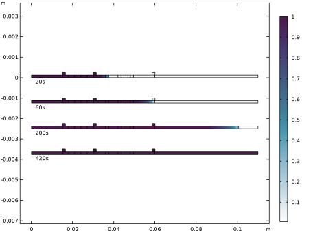
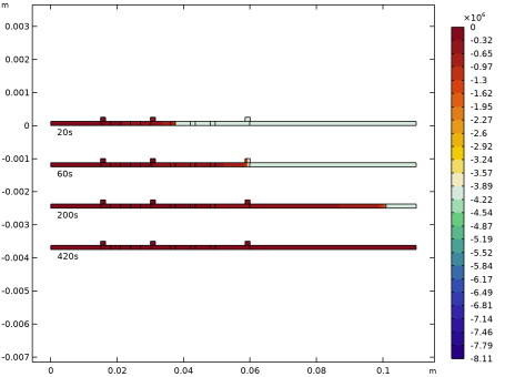
In the tree, select Study 1/Solution 1 (sol1) > Richards’ Equation > Pressure (dl) and Study 1/Solution 1 (sol1) > Richards’ Equation > Effective Saturation (dl).
4
Click the Add Result Template button in the window toolbar.
5
In the Results toolbar, click  Result Templates to close the Result Templates window.
Results
Pressure (dl)
1
In the Model Builder window, expand the Results > Pressure (dl) node, then click Pressure (dl).
2
In the Settings window for 2D Plot Group, click to expand the Title section.
3
From the Title type list, choose None.
4
Click to expand the Plot Array section. From the Array type list, choose Linear.
5
From the Array axis list, choose y.
6
From the Displacement list, choose Absolute.
7
In the Cell displacement text field, type -1.25e-3.
Solution Array 1
1
In the Model Builder window, right-click Surface and choose Solution Array.
2
In the Settings window for Solution Array, locate the Data section.
3
From the Time selection list, choose Interpolated.
4
In the Times (s) text field, type 20 60 200 420.
5
In the Pressure (dl) toolbar, click  Plot.
6
Click the  Zoom Extents button in the Graphics toolbar.
Pressure (dl)
In the Pressure (dl) toolbar, click  More Plots and choose Table Annotation.
Table Annotation 1
1
In the Settings window for Table Annotation, locate the Data section.
2
From the Source list, choose Local table.
3
4
Locate the Coloring and Style section. Clear the Show point checkbox.
Pressure (dl)
1
In the Model Builder window, click Pressure (dl).
2
In the Pressure (dl) toolbar, click  Plot.
Effective Saturation (dl)
1
In the Model Builder window, expand the Results > Effective Saturation (dl) node, then click Effective Saturation (dl).
2
In the Settings window for 2D Plot Group, locate the Title section.
3
From the Title type list, choose None.
4
Locate the Plot Array section. From the Array type list, choose Linear.
5
From the Array axis list, choose y.
6
From the Displacement list, choose Absolute.
7
In the Cell displacement text field, type -1.25e-3.
Solution Array 1
1
In the Model Builder window, right-click Surface 1 and choose Solution Array.
2
In the Settings window for Solution Array, locate the Data section.
3
From the Time selection list, choose Interpolated.
4
In the Times (s) text field, type 20 60 200 420.
Table Annotation 1
In the Model Builder window, under Results > Pressure (dl) right-click Table Annotation 1 and choose Copy.
Table Annotation 1
1
In the Model Builder window, right-click Effective Saturation (dl) and choose Paste Table Annotation.
2
In the Effective Saturation (dl) toolbar, click  Plot.
3
Click the  Zoom Extents button in the Graphics toolbar.
Component 1 (comp1)
Next, set up the chemical reactions together with mass transport. If available in your license, the Chemistry interface provides a convenient way to define reactions. In this model, the Domain, ODEs and DAEs interface is used. For convenience, a fully set-up interface is imported from an external file.
1
In the Home toolbar, click Insert Physics and choose Insert Physics.
2
In the Insert Physics dialog, click  Browse.
3
4
Inspect the Reactions node (the Domain ODEs and DAEs interface). Eight species and hence eight dependent variables are defined. For each section of the detection test, a domain feature specifies the reactions described in Chemical Reactions. Some variables are still undefined at this stage, namely the species that are transported. These will be introduced in the next step, when setting up the transport interface.
Add Physics
1
In the Home toolbar, click  Windows and choose Add Physics.
2
Go to the Add Physics window.
3
In the tree, select Chemical Species Transport > Transport of Diluted Species in Porous Media (tds).
4
Find the Physics interfaces in study subsection. In the table, clear the Solve checkbox for Study 1 as the chemical reactions and transport variables will be solved for in a different study.
5
Click the Add to Component 1 button in the window toolbar.
6
In the Home toolbar, click  Add Physics to close the Add Physics window.
Transport of Diluted Species in Porous Media (tds)
1
In the Settings window for Transport of Diluted Species in Porous Media, click to expand the Discretization section.
2
From the Concentration list, choose Quadratic.
3
Click to expand the Dependent Variables section. In the Number of species text field, type 6.
4
In the Concentrations (mol/m³) table, enter the following settings:
Fluid 1
1
In the Model Builder window, under Component 1 (comp1) > Transport of Diluted Species in Porous Media (tds) > Porous Medium 1 click Fluid 1.
2
In the Settings window for Fluid, locate the Convection section.
3
From the u list, choose Total Darcy velocity field (dl/usporous1).
4
Locate the Diffusion section. In the DF,cIgM text field, type D1.
5
In the DF,cIgMC text field, type D1.
6
In the DF,cIgG text field, type D1.
7
In the DF,cIgGC text field, type D1.
8
In the DF,cAA text field, type D1.
9
In the DF,cAAC text field, type D1.
10
From the Effective diffusivity model list, choose No correction.
Inflow 1
1
In the Physics toolbar, click  Boundaries and choose Inflow.
2
3
In the Settings window for Inflow, locate the Concentration section.
4
In the c0,cIgM text field, type c0*step1(t).
5
In the c0,cIgG text field, type c0*step1(t).
6
In the c0,cAA text field, type c0*step1(t).
Definitions (comp1)
Add the reactions for the different conjugation pad areas and test lines. First, define the reaction variables.
Variables: Reaction Rates
1
In the Model Builder window, under Component 1 (comp1) right-click Definitions and choose Variables.
2
In the Settings window for Variables, type Variables: Reaction Rates in the Label text field.
3
Locate the Variables section. Click  Load from File.
4
Browse to the model’s Application Libraries folder and double-click the file rapid_detection_test_2d_variables_reaction_rates.txt.
Transport of Diluted Species in Porous Media (tds)
Reactions: Antibody Binding
1
In the Physics toolbar, click  Domains and choose Reactions.
2
In the Settings window for Reactions, type Reactions: Antibody Binding in the Label text field.
3
Locate the Domain Selection section. From the Selection list, choose Antibody Binding.
4
Locate the Reaction Rates section. In the RcIgM text field, type -r_IgMC.
5
In the RcIgMC text field, type r_IgMC.
6
In the RcIgG text field, type -r_IgGC.
7
In the RcIgGC text field, type r_IgGC.
Reactions: Animal Antibodies
1
In the Physics toolbar, click  Domains and choose Reactions.
2
In the Settings window for Reactions, type Reactions: Animal Antibodies in the Label text field.
3
Locate the Domain Selection section. From the Selection list, choose Animal Antibodies.
4
Locate the Reaction Rates section. In the RcAA text field, type -r_AAC.
5
In the RcAAC text field, type r_AAC.
Reactions: IgM Detection
1
In the Physics toolbar, click  Domains and choose Reactions.
2
In the Settings window for Reactions, type Reactions: IgM Detection in the Label text field.
3
Locate the Domain Selection section. From the Selection list, choose IgM Detection.
4
Locate the Reaction Rates section. In the RcIgMC text field, type -r_IgMPos.
Reactions: IgG Detection
1
In the Physics toolbar, click  Domains and choose Reactions.
2
In the Settings window for Reactions, type Reactions: IgG Detection in the Label text field.
3
Locate the Domain Selection section. From the Selection list, choose IgG Detection.
4
Locate the Reaction Rates section. In the RcIgGC text field, type -r_IgGPos.
Reactions: Antigen Detection
1
In the Physics toolbar, click  Domains and choose Reactions.
2
In the Settings window for Reactions, type Reactions: Antigen Detection in the Label text field.
3
Locate the Domain Selection section. From the Selection list, choose Antigen Detection.
4
Locate the Reaction Rates section. In the RcAAC text field, type -r_AAPos.
Add Study
1
In the Home toolbar, click  Windows and choose Add Study.
2
Go to the Add Study window.
3
Find the Physics interfaces in study subsection. In the table, clear the Solve checkboxes for Richards’ Equation (dl) and Events (ev).
4
Find the Studies subsection. In the Select Study tree, select General Studies > Time Dependent.
5
Click the Add Study button in the window toolbar.
6
In the Home toolbar, click  Add Study to close the Add Study window.
Study 2
Step 1: Time Dependent
1
In the Settings window for Time Dependent, locate the Study Settings section.
2
In the Output times text field, type 5*(exp(range(0,1/19,1)*4)-1)/(exp(4)-1) range(10,5,420).
3
Locate the Results While Solving section. From the Probes list, choose None.
4
In the Model Builder window, click Study 2.
5
In the Settings window for Study, locate the Study Settings section.
6
Clear the Generate default plots checkbox.
7
In the Model Builder window, click Step 1: Time Dependent.
8
In the Settings window for Time Dependent, click to expand the Values of Dependent Variables section.
9
Find the Values of variables not solved for subsection. From the Settings list, choose User controlled.
10
From the Method list, choose Solution.
11
From the Study list, choose Study 1, Time Dependent.
12
From the Time (s) list, choose Automatic (all solutions).
For each time step in the transport and reaction simulation, the corresponding solution from Richards’ Equation is retrieved.
Solution 2 (sol2)
1
In the Study toolbar, click  Show Default Solver.
2
In the Model Builder window, expand the Solution 2 (sol2) node, then click Dependent Variables 1.
3
In the Settings window for Dependent Variables, locate the Scaling section.
4
From the Method list, choose Manual.
5
In the Model Builder window, under Study 2 > Solver Configurations > Solution 2 (sol2) click Time-Dependent Solver 1.
6
In the Settings window for Time-Dependent Solver, locate the Time Stepping section.
7
From the Steps taken by solver list, choose Strict.
8
Find the Algebraic variable settings subsection. From the Consistent initialization list, choose Off.
9
In the Study toolbar, click  Compute.
Study 1
In case you want to rerun the first study, the reactions need to be deactivated there.
Step 1: Time Dependent
1
In the Model Builder window, under Study 1 click Step 1: Time Dependent.
2
In the Settings window for Time Dependent, locate the Physics and Variables Selection section.
3
In the Solve for column of the table, under Component 1 (comp1), clear the checkbox for Reactions (dode).
Results
To plot the different antibody concentrations, follow the steps below.
IgMC Concentration
1
In the Results toolbar, click  2D Plot Group.
2
In the Settings window for 2D Plot Group, type IgMC Concentration in the Label text field.
Surface 1
Right-click IgMC Concentration and choose Surface.
IgMC Concentration
Locate the Data section. From the Dataset list, choose Study 2/Solution 2 (sol2).
Surface 1
1
In the Model Builder window, click Surface 1.
2
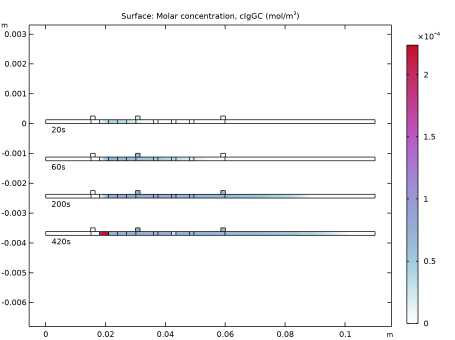
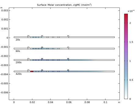
In the Settings window for Surface, click Replace Expression in the upper-right corner of the Expression section. From the menu, choose Component 1 (comp1) > Transport of Diluted Species in Porous Media > Species cIgMC > cIgMC - Molar concentration, cIgMC - mol/m³.
3
Locate the Coloring and Style section. From the Color table list, choose Acanthaster.
Solution Array 1
1
Right-click Surface 1 and choose Solution Array.
2
In the Settings window for Solution Array, locate the Data section.
3
From the Time selection list, choose Interpolated.
4
In the Times (s) text field, type 20 60 200 420.
IgMC Concentration
1
In the Model Builder window, under Results click IgMC Concentration.
2
In the Settings window for 2D Plot Group, locate the Plot Array section.
3
From the Array axis list, choose y.
4
From the Displacement list, choose Absolute.
5
In the Cell displacement text field, type -1.25e-3.
Table Annotation 1
1
In the IgMC Concentration toolbar, click  More Plots and choose Table Annotation.
2
In the Settings window for Table Annotation, locate the Data section.
3
From the Source list, choose Local table.
4
5
Locate the Coloring and Style section. Clear the Show point checkbox.
IgMC Concentration
1
In the Model Builder window, click IgMC Concentration.
2
In the Settings window for 2D Plot Group, locate the Title section.
3
From the Title type list, choose Custom.
4
Find the Solution subsection. Clear the Solution checkbox.
5
In the IgMC Concentration toolbar, click  Plot.
6
Click the  Zoom Extents button in the Graphics toolbar.
IgGC Concentration
1
Right-click IgMC Concentration and choose Duplicate.
2
In the Model Builder window, click IgMC Concentration 1.
3
In the Settings window for 2D Plot Group, type IgGC Concentration in the Label text field.
Surface 1
1
In the Model Builder window, click Surface 1.
2
In the Settings window for Surface, locate the Expression section.
3
In the Expression text field, type cIgGC.
4
In the IgGC Concentration toolbar, click  Plot.
AAC Concentration
1
In the Model Builder window, right-click IgGC Concentration and choose Duplicate.
2
In the Model Builder window, click IgGC Concentration 1.
3
In the Settings window for 2D Plot Group, type AAC Concentration in the Label text field.
Surface 1
1
In the Model Builder window, click Surface 1.
2
In the Settings window for Surface, locate the Expression section.
3
In the Expression text field, type cAAC.
4
In the AAC Concentration toolbar, click  Plot.
Continue with plotting the number of particles per unit surface as in Figure 8 which indicates the visibility of the test line.
Evaluation Group: Test Line
1
In the Results toolbar, click  Evaluation Group.
2
In the Settings window for Evaluation Group, type Evaluation Group: Test Line in the Label text field.
3
Locate the Data section. From the Dataset list, choose Study 2/Solution 2 (sol2).
Surface Average 1
1
Right-click Evaluation Group: Test Line and choose Average > Surface Average.
2
In the Settings window for Surface Average, locate the Selection section.
3
From the Selection list, choose IgM Detection.
4
Locate the Expressions section. Click  Clear Table.
5
Surface Average 2
1
Right-click Surface Average 1 and choose Duplicate.
2
In the Settings window for Surface Average, locate the Expressions section.
3
4
Locate the Selection section. From the Selection list, choose IgG Detection.
Surface Average 3
1
Right-click Surface Average 2 and choose Duplicate.
2
In the Settings window for Surface Average, locate the Selection section.
3
From the Selection list, choose Antigen Detection.
4
Locate the Expressions section. In the table, enter the following settings:
Evaluation Group: Test Line
1
In the Model Builder window, click Evaluation Group: Test Line.
2
In the Evaluation Group: Test Line toolbar, click  Evaluate.
Evaluation Group: Test Line
1
Go to the Evaluation Group: Test Line window.
2
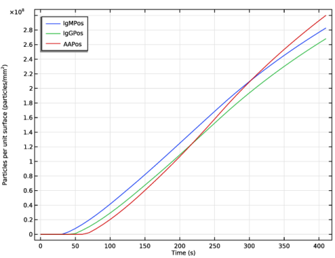
Click the Table Graph button in the window toolbar.
Results
Table Graph 1
1
In the Settings window for Table Graph, click to expand the Legends section.
2
Select the Show legends checkbox.
3
From the Legends list, choose Manual.
4
Concentration, IgMPos, IgGPos, AAPos
1
In the Model Builder window, click 1D Plot Group 6.
2
In the Settings window for 1D Plot Group, locate the Legend section.
3
From the Position list, choose Upper left.
4
Locate the Plot Settings section.
5
Select the y-axis label checkbox. In the associated text field, type Particles per unit surface (mm<sup>2</sup>).
6
Click to expand the Title section. From the Title type list, choose Manual.
7
In the Label text field, type Concentration, IgMPos, IgGPos, AAPos.
8
Locate the Title section. From the Title type list, choose None.
9
Click the  Zoom Extents button in the Graphics toolbar.
10
In the Concentration, IgMPos, IgGPos, AAPos toolbar, click  Plot.