PDF

Estimating Permeability from Microscale Porous Structures
Introduction
This tutorial model demonstrates how to compute porosity and permeability of a sphere packing from a fully resolved microscopic model. These values are then used to model the sphere packing on the macroscopic scale using Darcy’s Law.
Model Definition
The geometry used to calculate the permeability in the microscopic scale is shown in the figure below.
Figure 1: Geometry of the unit cell of a sphere packing.
A body-centered cubic (BCC) lattice is used. The flow around the spheres is described using the Creeping Flow interface. A pressure difference of 1 Pa is applied. The boundaries that correspond to the solid-fluid interface are defined as walls and the remaining boundaries are symmetry boundaries.
From this set up the porosity and permeability can be calculated. The porosity is defined as the fraction of pore space volume Vfluid to total volume Vtot
.
To calculate the permeability κ (m2) the following relationship is used
whereas the pressure gradient p is replaced by the pressure drop across the unit divided by the size of the unit cell L and the velocity vector u is replaced by the normal velocity uout in flow direction (z direction), hence
.
The computation is carried out for a range of porosities, and the resulting permeability values are used to determine a power-law relationship using the Least-Squares Fit method. The power law takes the form:
(1)
with the coefficients b and n to be computed from the fit.
To verify that a macroscopic approach using homogenization by deploying Darcy’s Law gives accurate values, the model compares the mass flow per unit area (
L2).
Results and Discussion
The velocity field in the unit cell is shown in Figure 2.
Figure 2: Velocity in the unit cell.
The Least-Squares Fit (Figure 3) results in b = 7.3e-9 and n = 4.2.
Figure 3: Computed results (gray squares) and fitted function (blue line).
Figure 4 shows the pressure distribution in the macroscopic model.
Figure 4: Pressure field for the macroscopic model.
To compare the accuracy of the power law model with the pore-scale model, the normal mass flow is computed and compared. The results are in good agreement (Figure 5).
Figure 5: Normal mass flow (outflow) for different porosities compared.
Notes About the COMSOL Implementation
To generate the geometry of the unit cell of a sphere packing the COMSOL Multiphysics Part Libraries can be used. They contain sets of common parts or components that can simplify and streamline the construction of more complex geometries. The part library Representative Volume Elements offers several geometry parts for 2D and 3D geometries to choose from.
Application Library path: Porous_Media_Flow_Module/Fluid_Flow/permeability_estimation
Modeling Instructions
From the File menu, choose New.
New
In the New window, click  Model Wizard.
Model Wizard
1
In the Model Wizard window, click  3D.
2
In the Select Physics tree, select Fluid Flow > Single-Phase Flow > Creeping Flow (spf).
3
Click Add.
4
Click  Study.
5
In the Select Study tree, select General Studies > Stationary.
6
Start setting up the model by defining some geometry parameters as the particle diameter, particle distance, and side length of the unit cell.
Global Definitions
Parameters 1
1
In the Model Builder window, under Global Definitions click Parameters 1.
2
In the Settings window for Parameters, locate the Parameters section.
3
Geometry 1
Now choose a representative volume element from the COMSOL Multiphysics part libraries and adjust it as desired.
Part Libraries
1
From the Windows menu, choose Part Libraries.
2
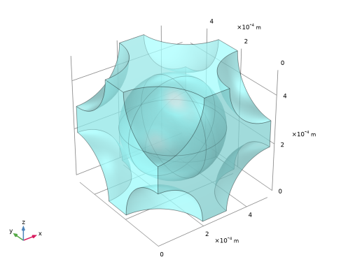
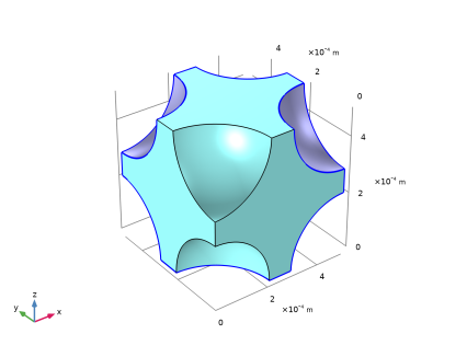
In the Part Libraries window, select COMSOL Multiphysics > Unit Cells and RVEs > Particulate Composites > particulate_body_centered_cubic in the tree.
3
Click  Add to Geometry.
4
In the Select Part Variant dialog, select Specify particle volume fraction in the Select part variant list.
5
Geometry 1
Particulate Composite, Body-Centered Cubic 1 (pi1)
1
In the Model Builder window, expand the Geometry 1 node, then click Particulate Composite, Body-Centered Cubic 1 (pi1).
2
In the Settings window for Part Instance, locate the Input Parameters section.
3
The part comes with predefined selections. Only keep the selections that are used for the physics setup. This is optional.
4
Click to expand the Boundary Selections section. In the table, clear the Keep checkboxes for Pair 1, Source, Pair 1, Destination, Pair 2, Source, Pair 2, Destination, Pair 3, Source, Pair 3, Destination, Pair 1, Pair 2, and Interior.
Extract 1 (extract1)
1
In the Geometry toolbar, click  Extract.
2
In the Settings window for Extract, locate the Entities or Objects to Extract section.
3
From the Geometric entity level list, choose Domain.
4
From the Input object handling list, choose Remove.
5
On the object pi1, select Domain 2 only.
6
Click  Build All Objects. Compare the geometry with Figure 1.
Create a selection for the symmetry boundaries.
Symmetry
1
In the Geometry toolbar, click  Selections and choose Difference Selection.
2
In the Settings window for Difference Selection, locate the Geometric Entity Level section.
3
From the Level list, choose Boundary.
4
Locate the Input Entities section. Click the  Add button for Selections to add.
5
In the Add dialog, select Exterior (Particulate Composite, Body-Centered Cubic 1) in the Selections to add list.
6
7
In the Settings window for Difference Selection, locate the Input Entities section.
8
Click the  Add button for Selections to subtract.
9
In the Add dialog, select Pair 3 (Particulate Composite, Body-Centered Cubic 1) in the Selections to subtract list.
10
11
In the Settings window for Difference Selection, type Symmetry in the Label text field.
Global Definitions
Add some parameters to the Parameters list, that are used to set up the physics.
Parameters 1
1
In the Model Builder window, under Global Definitions click Parameters 1.
2
In the Settings window for Parameters, locate the Parameters section.
3
Materials
Material 1 (mat1)
1
In the Model Builder window, under Component 1 (comp1) right-click Materials and choose Blank Material.
2
In the Settings window for Material, locate the Material Contents section.
3
Creeping Flow (spf)
Periodic Flow Condition 1
1
In the Physics toolbar, click  Boundaries and choose Periodic Flow Condition.
2
In the Settings window for Periodic Flow Condition, locate the Boundary Selection section.
3
From the Selection list, choose Pair 3 (Particulate Composite, Body-Centered Cubic 1).
4
Locate the Flow Condition section. In the Δp text field, type p0.
Symmetry 1
1
In the Physics toolbar, click  Boundaries and choose Symmetry.
2
In the Settings window for Symmetry, locate the Boundary Selection section.
3
From the Selection list, choose Symmetry.
Currently, the system is underconstrained because only the pressure difference is known, not the absolute pressure. To obtain a unique solution, fix the pressure at one point.
Pressure Point Constraint 1
1
In the Physics toolbar, click  Points and choose Pressure Point Constraint.
2
Define an integration variable to calculate the normal velocity at the destination end of the periodic condition.
Definitions
Integration 1 (intop1)
1
In the Definitions toolbar, click  Nonlocal Couplings and choose Integration.
2
In the Settings window for Integration, locate the Source Selection section.
3
From the Geometric entity level list, choose Boundary.
4
Variables 1
1
In the Model Builder window, right-click Definitions and choose Variables.
2
In the Settings window for Variables, locate the Variables section.
3
Mesh 1
The physics-controlled mesh sets up a boundary layer mesh at the walls which ensures a good resolution of the steep velocity gradients in that region.
1
In the Model Builder window, under Component 1 (comp1) click Mesh 1.
2
In the Settings window for Mesh, locate the Physics-Controlled Mesh section.
3
From the Element size list, choose Fine.
4
In the table, clear the Use checkbox for Geometric Analysis, Detail Size.
5
Click  Build All.
Study 1
Perform a parametric sweep over the particle volume fraction to determine the power-law relationship between porosity and permeability
Parametric Sweep
1
In the Study toolbar, click  Parametric Sweep.
2
In the Settings window for Parametric Sweep, locate the Study Settings section.
3
4
5
Click  Range.
6
In the Range dialog, type 0.3 in the Start text field.
7
In the Step text field, type 0.1.
8
In the Stop text field, type 0.6.
9
Click Replace.
10
In the Model Builder window, click Study 1.
11
In the Settings window for Study, locate the Study Settings section.
12
Clear the Generate default plots checkbox, to disable the automatic generation of default plots. Instead, choose the relevant plots from the Result Templates after computation.
13
In the Study toolbar, click  Compute.
Result Templates
Add and modify the velocity plot to obtain Figure 2.
1
In the Results toolbar, click  Result Templates to open the Result Templates window.
2
Go to the Result Templates window.
3
In the tree, select Study 1/Solution 1 (sol1) > Creeping Flow > Velocity (spf).
4
Click the Add Result Template button in the window toolbar.
5
In the Results toolbar, click  Result Templates to close the Result Templates window.
Results
Multislice 1
1
In the Model Builder window, expand the Velocity (spf) node, then click Multislice 1.
2
In the Settings window for Multislice, locate the Coloring and Style section.
3
From the Color table list, choose Acanthaster.
Surface 1
1
In the Model Builder window, right-click Velocity (spf) and choose Surface.
2
In the Settings window for Surface, locate the Expression section.
3
In the Expression text field, type 1.
4
Locate the Coloring and Style section. From the Coloring list, choose Uniform.
5
From the Color list, choose Gray.
Selection 1
1
Right-click Surface 1 and choose Selection.
2
In the Settings window for Selection, locate the Selection section.
3
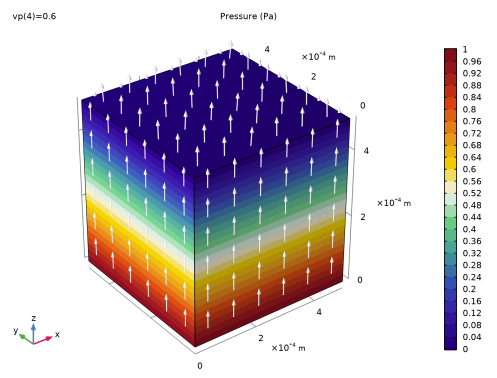
From the Selection list, choose All boundaries and remove the top, bottom and front boundaries as shown below.
Streamline 1
1
In the Model Builder window, right-click Velocity (spf) and choose Streamline.
2
3
In the Settings window for Streamline, locate the Streamline Positioning section.
4
In the Number text field, type 40.
5
Locate the Coloring and Style section. Find the Point style subsection. From the Type list, choose Arrow.
6
Select the Number of arrows checkbox. In the associated text field, type 80.
7
In the Velocity (spf) toolbar, click  Plot.
Color Expression 1
1
Right-click Streamline 1 and choose Color Expression.
2
In the Settings window for Color Expression, locate the Expression section.
3
In the Expression text field, type p.
4
Locate the Coloring and Style section. From the Color table list, choose GrayPrint.
Velocity (spf)
1
In the Model Builder window, under Results click Velocity (spf).
2
In the Settings window for 3D Plot Group, locate the Data section.
3
From the Dataset list, choose Study 1/Parametric Solutions 1 (sol2).
4
From the Parameter value (vp) list, choose 0.4.
5
Locate the Plot Settings section. Clear the Plot dataset edges checkbox.
6
Locate the Color Legend section. Select the Show units checkbox.
7
In the Velocity (spf) toolbar, click  Plot.
Compute the permeability for all parameters.
Global Evaluation 1
1
In the Results toolbar, click  Global Evaluation.
2
In the Settings window for Global Evaluation, locate the Data section.
3
From the Dataset list, choose Study 1/Parametric Solutions 1 (sol2).
4
Locate the Expressions section. In the table, enter the following settings:
5
Click  Evaluate. The results are written to a table.
Table 1
1
Go to the Table 1 window.
Compute the power-law parameters from the sweep results using a least-squares fit according to Equation 1.
Global Definitions
Least-Squares Fit 1 (lsq1_fun1)
1
In the Home toolbar, click  Functions and choose Global > Least-Squares Fit.
2
In the Settings window for Least-Squares Fit, locate the Data section.
3
From the Data source list, choose Result table.
4
Locate the Data Column Settings section. In the table, enter the following settings:
5
In the Expression text field, type b*x1^n.
6
Locate the Parameters section. In the table, enter the following settings:
7
Click  Fit Parameters.
Note, the results for b and n that appear in the Parameters section.
8
Click  Create Plot  and compare with Figure 3.
Results
Power Law Permeability
1
In the Settings window for 1D Plot Group, type Power Law Permeability in the Label text field.
2
Locate the Plot Settings section.
3
Select the x-axis label checkbox. In the associated text field, type Porosity.
4
Select the y-axis label checkbox. In the associated text field, type Permeability (m<sup>2</sup>.
5
In the Power Law Permeability toolbar, click  Plot.
6
Click to expand the Title section. From the Title type list, choose None.
Root
Now, add a new component to set up a Darcy’s Law interface and use these values.
Add Component
In the Model Builder window, right-click the root node and choose Add Component > 3D.
Geometry 2
Block 1 (blk1)
1
In the Geometry toolbar, click  Block.
2
In the Settings window for Block, locate the Size and Shape section.
3
In the Width text field, type L.
4
In the Depth text field, type L.
5
In the Height text field, type L.
6
Click  Build All Objects.
Add Physics
1
In the Home toolbar, click  Add Physics to open the Add Physics window.
2
Go to the Add Physics window.
3
In the tree, select Fluid Flow > Porous Media and Subsurface Flow > Darcy’s Law (dl).
4
Find the Physics interfaces in study subsection. In the table, clear the Solve checkbox for Study 1.
5
Click the Add to Component 2 button in the window toolbar.
6
In the Home toolbar, click  Add Physics to close the Add Physics window.
Darcy’s Law (dl)
Fluid 1
1
In the Settings window for Fluid, locate the Fluid Properties section.
2
From the ρ list, choose User defined. In the associated text field, type rho_f.
3
From the μ list, choose User defined. In the associated text field, type mu_f.
Porous Matrix 1
1
In the Model Builder window, click Porous Matrix 1.
2
In the Settings window for Porous Matrix, locate the Matrix Properties section.
3
From the εp list, choose User defined. In the associated text field, type por.
4
From the Permeability model list, choose Power law.
5
In the bPL text field, type lsq1.b.
6
In the nPL text field, type lsq1.n.
Note, that lsqq1. refers to the Least-Squares Fit function.
Periodic Condition 1
1
In the Physics toolbar, click  Boundaries and choose Periodic Condition.
2
3
In the Settings window for Periodic Condition, locate the Flow Condition section.
4
In the Δp text field, type p0.
Again, the system is underconstrained. Darcy’s Law does not include a predefined pressure constraint, but a general constraint can be applied just as easily.
5
Click the  Show More Options button in the Model Builder toolbar.
6
In the Show More Options dialog, in the tree, select the checkbox for the node Physics > Equation Contributions.
7
Constraint 2
1
In the Physics toolbar, click  Points and choose Constraint.
2
3
In the Settings window for Constraint, locate the Constraint section.
4
In the Constraint expression text field, type p2.
Note, that you need to type the variable to be constrained.
Add Study
1
In the Home toolbar, click  Add Study to open the Add Study window.
2
Go to the Add Study window.
3
Find the Studies subsection. In the Select Study tree, select General Studies > Stationary.
4
Disable the Creeping Flow interface for this study.
5
Click the Add Study button in the window toolbar.
6
In the Home toolbar, click  Add Study to close the Add Study window.
Study 2
Parametric Sweep
1
In the Study toolbar, click  Parametric Sweep.
2
In the Settings window for Parametric Sweep, locate the Study Settings section.
3
4
5
6
In the Model Builder window, click Study 2.
7
In the Settings window for Study, locate the Study Settings section.
8
Clear the Generate default plots checkbox, to disable the automatic generation of default plots. Instead, choose the relevant plots from the Result Templates after computation.
9
In the Study toolbar, click  Compute.
Result Templates
Add and modify the pressure plot to obtain Figure 4.
1
In the Results toolbar, click  Result Templates to open the Result Templates window.
2
Go to the Result Templates window.
3
In the tree, select Study 2/Parametric Solutions 2 (6) (sol8) > Darcy’s Law > Pressure (dl).
4
Click the Add Result Template button in the window toolbar.
5
In the Results toolbar, click  Result Templates to close the Result Templates window.
Results
Arrow Surface 1
1
In the Model Builder window, right-click Pressure (dl) and choose Arrow Surface.
2
In the Settings window for Arrow Surface, click to expand the Title section.
3
From the Title type list, choose None.
4
Locate the Coloring and Style section. From the Color list, choose White.
5
In the Pressure (dl) toolbar, click  Plot.
Finally, compare the models using the normal mass flow.
Global Evaluation 2
1
In the Results toolbar, click  Global Evaluation.
2
In the Settings window for Global Evaluation, locate the Data section.
3
From the Dataset list, choose Study 1/Parametric Solutions 1 (sol2).
4
Locate the Expressions section. In the table, enter the following settings:
5
Clicknext to  Evaluate, then choose New Table.
Surface Integration 1
1
In the Model Builder window, right-click Derived Values and choose Integration > Surface Integration.
2
In the Settings window for Surface Integration, locate the Data section.
3
From the Dataset list, choose Study 2/Parametric Solutions 2 (6) (sol8).
4
5
Click Replace Expression in the upper-right corner of the Expressions section. From the menu, choose Component 2 (comp2) > Darcy’s Law > Boundary fluxes > dl.bndflux - Boundary flux - kg/(m²·s).
6
Clicknext to  Evaluate, then choose Table 2 - Global Evaluation 2.
Table 2
1
Go to the Table 2 window.
2
Click the Table Graph button in the window toolbar.
Results
1D Plot Group 4
1
In the Model Builder window, under Results click 1D Plot Group 4.
2
In the Settings window for 1D Plot Group, locate the Plot Settings section.
3
Select the x-axis label checkbox. In the associated text field, type Particle Volume Fraction.
4
Select the y-axis label checkbox. In the associated text field, type Mass Flow.
Table Graph 1
1
In the Model Builder window, click Table Graph 1.
2
In the Settings window for Table Graph, click to expand the Legends section.
3
Select the Show legends checkbox.
4
From the Legends list, choose Manual.
5
1D Plot Group 4
1
In the Model Builder window, click 1D Plot Group 4.
2
In the 1D Plot Group 4 toolbar, click  Plot  and compare with Figure 5. The results are in good agreement.