
|
|
|

 .
. .
.
|
1
|
|
2
|
|
3
|
Click Add.
|
|
4
|
Click
|
|
5
|
|
6
|
Click
|
|
1
|
|
2
|
|
3
|
Click
|
|
4
|
Browse to the model’s Application Libraries folder and double-click the file mandel_cryer_effect_parameters.txt.
|
|
1
|
|
2
|
|
3
|
|
4
|
|
5
|
Click
|
|
6
|
|
1
|
|
1
|
|
1
|
|
3
|
|
4
|
|
5
|
|
1
|
|
2
|
|
3
|
|
4
|
Click to collapse the Discretization section.
|
|
1
|
|
1
|
|
3
|
|
4
|
|
1
|
|
3
|
In the Settings window for Porous Medium, type Porous Medium: Kozeny-Carman in the Label text field.
|
|
1
|
|
2
|
|
3
|
|
4
|
|
1
|
In the Model Builder window, expand the Component 1 (comp1) > Multiphysics > Poroelasticity 1 (poro1) node, then click Poroelasticity 1 (poro1).
|
|
2
|
|
3
|
|
4
|
|
1
|
In the Model Builder window, expand the Component 1 (comp1) > Materials > Porous Material 1 (pmat1) node, then click Porous Material 1 (pmat1).
|
|
2
|
|
3
|
Click
|
|
1
|
|
2
|
|
1
|
|
2
|
|
3
|
|
1
|
|
2
|
|
1
|
|
2
|
|
3
|
|
4
|
Click
|
|
1
|
|
2
|
|
3
|
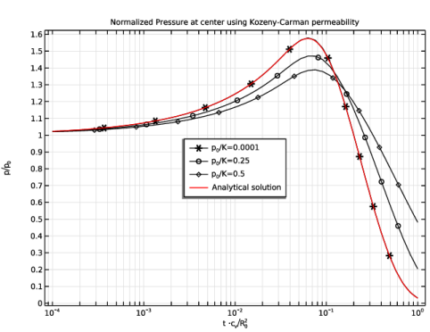
In the Output times text field, type 10^{range(-4,4/50,0)}* R0^2/cv. This input corresponds to the expected time dependency as shown in Equation 1, enforcing small time intervals in the beginning which are then exponentially growing. The end time of the study time interval is calculated as the square of the sphere radius divided by the coefficient of consolidation.
|
|
4
|
|
5
|
|
6
|
Clear the Generate default plots checkbox.
|
|
1
|
|
2
|
|
3
|
Click
|
|
5
|
|
6
|
In the Settings window for Study, type Study with Kozeny-Carman Permeability in the Label text field.
|
|
7
|
|
1
|
|
2
|
|
3
|
|
4
|
Click
|
|
5
|
Browse to the model’s Application Libraries folder and double-click the file mandel_cryer_effect_p_analytical.txt.
|
|
6
|
|
7
|
|
8
|
|
9
|
|
10
|
In the Argument table, enter the following settings:
|
|
1
|
|
2
|
|
3
|
|
4
|
|
5
|
|
6
|
|
7
|
|
8
|
|
9
|
|
10
|
|
1
|
|
2
|
|
3
|
|
4
|
|
5
|
|
6
|
|
7
|
|
8
|
Locate the Plot Settings section.
|
|
9
|
Select the x-axis label checkbox. In the associated text field, type t \cdot \[\mathrm{c_{v} / R_{0}^{2}}\], which is LaTex-syntax to write mathematical formulas and expressions.
|
|
10
|
|
11
|
|
1
|
|
3
|
|
4
|
|
5
|
|
6
|
|
7
|
|
8
|
|
9
|
|
10
|
|
11
|
|
12
|
|
1
|
In the Normalized Pressure (Kozeny-Carman Permeability) toolbar, click
|
|
2
|
|
3
|
|
4
|
Click Replace Expression in the upper-right corner of the y-Axis Data section. From the menu, choose Global definitions > Functions > p_analytical(t) - Analytical Solution.
|
|
5
|
|
6
|
|
7
|
|
8
|
|
9
|
|
11
|
|
12
|
|
13
|
|
1
|
|
2
|
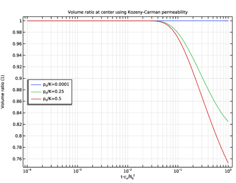
In the Settings window for 1D Plot Group, type Volume Ratio (Kozeny-Carman Permeability) in the Label text field.
|
|
3
|
Locate the Data section. From the Dataset list, choose Study with Kozeny-Carman Permeability/Parametric Solutions 1 (sol2).
|
|
4
|
Locate the Plot Settings section.
|
|
5
|
Select the x-axis label checkbox. In the associated text field, type t\cdot c\[_{\mathrm{v}}/\mathrm{R_{0}}^{2}\].
|
|
6
|
|
7
|
|
1
|
|
3
|
|
4
|
|
5
|
|
6
|
|
7
|
|
8
|
|
1
|
|
2
|
|
3
|
|
4
|
|
5
|
|
1
|
In the Model Builder window, under Component 1 (comp1) > Materials > Porous Material 1 (pmat1) click Basic (def).
|
|
2
|
|
3
|
Click
|
|
4
|
|
5
|
Click OK.
|
|
6
|
|
1
|
|
2
|
Go to the Add Study window.
|
|
3
|
|
4
|
Click the Add Study button in the window toolbar.
|
|
5
|
|
1
|
|
2
|
Clear the Generate default plots checkbox.
|
|
3
|
|
1
|
|
2
|
|
3
|
|
4
|
Locate the Physics and Variables Selection section. Select the Modify model configuration for study step checkbox.
|
|
5
|
|
6
|
Right-click and choose Disable.
|
|
1
|
|
2
|
|
3
|
Click
|
|
5
|
|
1
|
In the Model Builder window, right-click Normalized Pressure (Kozeny-Carman Permeability) and choose Duplicate.
|
|
2
|
|
3
|
|
4
|
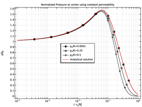
Locate the Title section. In the Title text area, type Normalized Pressure at center using constant permeability.
|
|
5
|
|
6
|
|
1
|
In the Model Builder window, right-click Volume Ratio (Kozeny-Carman Permeability) and choose Duplicate.
|
|
2
|
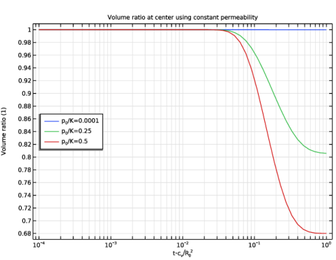
In the Settings window for 1D Plot Group, type Volume Ratio (Constant Permeability) in the Label text field.
|
|
3
|
Locate the Data section. From the Dataset list, choose Study with Constant Permeability/Parametric Solutions 2 (sol7).
|
|
4
|
Locate the Title section. In the Title text area, type Volume ratio at center using constant permeability.
|
|
5
|
|
1
|
|
2
|
Go to the Result Templates window.
|
|
3
|
In the tree, select Study with Kozeny-Carman Permeability/Parametric Solutions 1 (sol2) > Darcy’s Law > Pressure, 3D (dl).
|
|
4
|
Click the Add Result Template button in the window toolbar.
|
|
5
|
|
1
|
|
2
|
|
3
|
Click to expand the Advanced section. Locate the Plane Data section. From the Plane list, choose XY-planes.
|
|
4
|
Locate the Advanced section. Find the Space variables subsection. Select the Remove elements on the symmetry plane checkbox.
|
|
1
|
|
2
|
|
3
|
|
4
|
|
1
|
In the Model Builder window, expand the Pressure and Deformation (Kozeny-Carman Permeability) node, then click Surface.
|
|
2
|
|
3
|
|
4
|
Click to expand the Inherit Style section.
|
|
1
|
|
2
|
|
3
|
|
1
|
|
2
|
|
3
|
|
4
|
|
5
|
|
6
|
|
7
|
|
8
|
|
9
|
|
10
|
Clear the Arrow scale factor checkbox.
|
|
11
|
Clear the Color checkbox.
|
|
12
|
Clear the Color and data range checkbox.
|
|
13
|
Clear the Transparency checkbox.
|
|
1
|
|
2
|
|
3
|
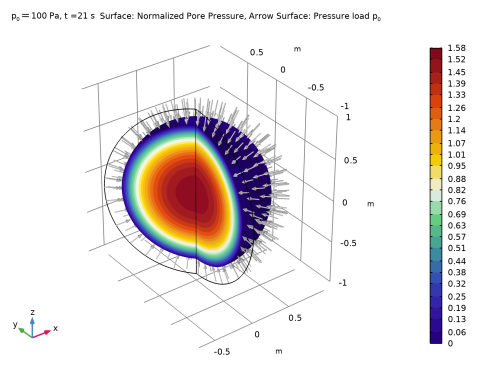
In the Title text area, type Surface: Normalized Pore Pressure, Arrow Surface: Pressure load p\[_{0}\].
|
|
4
|
|
5
|
|
6
|