PDF

Linear Biphasic Poroelasticity
Introduction
This example demonstrates how to use the Poroelasticity multiphysics coupling between the Solid Mechanics and Darcy’s Law interfaces to model linear biphasic poroviscoelastic behavior of soft biological tissues. Soft biological tissues are often modeled as biphasic materials with incompressible solid and fluid constituents. Note that even if both constituents are modeled as incompressible, the porous medium can still undergo large volume changes as a result of fluid inflow or outflow.
The implementation is verified using two numerical benchmarks from the literature, a torsion test and an indentation test on cylindrical plugs of articular cartilage.
Model Definition
The model consists of two components, one for the first benchmark test which is a torsion test, one for the second, which is an indentation test.
The first benchmark test, the infinitesimal torsion test, is used to determine the intrinsic viscoelastic behavior of the solid matrix under shear. The volume is preserved, so no pore pressure nor fluid flow develops. The design, a cylinder of 3 mm radius and 1.5 mm height, and operating conditions are taken from Ref. 1. Figure 1 shows a part of this cylinder. The arrows mark the tangential prescribed displacement. Due to rotational symmetry the problem can be reduced to modeling only the symmetry plane.
Figure 1: Full geometry and prescribed displacement of the torsion test (model component 1). The simulation is performed on the symmetry plane in 2D.
The second benchmark test is the indentation test, where the pore pressure contributes to the load, and volumetric changes in pore space affect the mass balance equation for the fluid. Again, due to rotational symmetry the simulation can be reduced to modeling only the symmetry plane. Figure 2 shows the model geometry and the prescribed indentation load.
Figure 2: Model geometry and indentation load for the second benchmark test. The simulation in performed on the symmetry plane in 2D.
In both cases, a linear isotropic viscoelastic material is used. The total stress σ in the tissue consists of the effective stress σe in the porous matrix and the pore pressure pf where
(1).
The effective stress contains both elastic and inelastic contributions; in this example, deviatoric and volumetric viscoelasticity are included based on Ref. 1. The viscoelastic behavior is described with a generalized Maxwell model.
The fluid permeation through the porous matrix is modeled by Darcy’s law.
(2)
where μ (Pa·s) is the fluid viscosity, κ (m2) the permeability of the porous substrate, and pf the pore pressure.
Results and Discussion
Figure 3 and Figure 4 show the results of the infinitesimal torsion test. Figure 3 shows the von Mises stress distribution over the surface of the cylindrical articular cartilage (color table) and the displacement, which is shown by the deformation of the cylinder. Stress and displacement are increasing with increasing distance from the rotation axis.
Figure 3: von Mises Stress (MPa) (colored) and tangential displacement (visible as deformation) along the surface of the cylindrical articular cartilage.
The torsional moment as a function of time is shown in Figure 4. The results calculated with COMSOL Multiphysics are shown in green, whereas the results of Ehlers and Markert (Ref. 1) are displayed as blue circles. The progression of the torsional moment indicates the characteristic fast stress relaxation of the organic solid matrix of cartilage tissues.
Figure 4: Torsional moment of the infinitesimal torsion test. The blue circles mark the results of Ehlers and Markert (2001), the green curve the results calculated with COMSOL Multiphysics.
Figure 5 and Figure 6 show the results of the second comparison, the indentation test.
Figure 5: Pore pressure at different loading ramp times.
Figure 5 displays the pore pressure within the model domain for different loading times. The deformation-dependent effect is restricted to the loaded area close to the singularity. In this region, the fluid flow is restrained causing a high local pore pressure. The indenter reaction force is shown in Figure 6. Both figures, especially Figure 6, show that the influence of the viscoelastic properties of the porous matrix decreases by increasing the loading time.
Figure 6: Indentation force as a function of time for different loading times (5 s, 100 s, and 250 s).
Reference
1. W. Ehlers and B. Markert, “A Linear Viscoelastic Biphasic Model for Soft Tissues Based on the Theory of Porous Media,” J. Biomech. Eng., vol. 123, pp. 418–424, 2001.
Application Library path: Porous_Media_Flow_Module/Verification_Examples/linear_biphasic_poroelasticity
Modeling Instructions
From the File menu, choose New.
New
In the New window, click  Model Wizard.
Model Wizard
1
In the Model Wizard window, click  2D Axisymmetric.
2
In the Select Physics tree, select Structural Mechanics > Solid Mechanics (solid).
3
Click Add.
4
Click  Study.
5
In the Select Study tree, select General Studies > Time Dependent.
6
Global Definitions
Load the parameters from separate external files for material parameters, torsion test parameters, and indentation test parameters. First, import the material parameters, which were defined according to Ref. 1.
Material Parameters
1
In the Model Builder window, under Global Definitions click Parameters 1.
2
In the Settings window for Parameters, type Material Parameters in the Label text field.
3
Locate the Parameters section. Click  Load from File.
4
Torsion Parameters
1
In the Home toolbar, click  Parameters and choose Add > Parameters.
2
In the Settings window for Parameters, type Torsion Parameters in the Label text field.
3
Locate the Parameters section. Click  Load from File.
4
Indentation Parameters
1
In the Home toolbar, click  Parameters and choose Add > Parameters.
2
In the Settings window for Parameters, type Indentation Parameters in the Label text field.
3
Locate the Parameters section. Click  Load from File.
4
In the next step, define the materials as global materials so that you can refer to them from different model components. Introduce them as empty material nodes; as soon as the physics has been defined the material node’s context menu will show you which properties are needed for the simulation. You can then just fill in the values defined in the Parameters list.
Solid Phase
1
In the Model Builder window, under Global Definitions right-click Materials and choose Blank Material.
2
In the Settings window for Material, type Solid Phase in the Label text field.
Fluid Phase
1
Right-click Materials and choose Blank Material.
2
In the Settings window for Material, type Fluid Phase in the Label text field.
Add a step function to use for applying the instantaneous twist in the torsion test case.
Step 1 (step1)
1
In the Home toolbar, click  Functions and choose Global > Step.
2
In the Settings window for Step, click to expand the Smoothing section.
3
Clear the Size of transition zone checkbox.
4
Click to expand the Plot Parameters section.
For the indentation test case, add a ramp function to ramp up the indentation displacement.
Ramp 1 (rm1)
1
In the Home toolbar, click  Functions and choose Global > Ramp.
2
In the Settings window for Ramp, locate the Parameters section.
3
Select the Cutoff checkbox.
4
Click to expand the Smoothing section. Click to expand the Plot Parameters section.
Now, set up the torsion load case.
Component 1: Torsion Test
1
In the Model Builder window, click Component 1 (comp1).
2
In the Settings window for Component, type Component 1: Torsion Test in the Label text field.
Geometry 1
1
In the Model Builder window, under Component 1: Torsion Test (comp1) click Geometry 1.
2
In the Settings window for Geometry, locate the Units section.
3
From the Length unit list, choose mm.
Rectangle 1 (r1)
1
In the Geometry toolbar, click  Rectangle.
2
In the Settings window for Rectangle, locate the Size and Shape section.
3
In the Width text field, type radius_t.
4
In the Height text field, type height_t.
5
Click  Build Selected.
Form Union (fin)
In the Geometry toolbar, click  Build All.
Materials
The volume is preserved in the torsion test case. Therefore, no pore pressure is developed and no fluid flow occurs, so only a solid material definition is needed. Link the local material to the globally defined one.
Material Link 1 (matlnk1)
In the Model Builder window, under Component 1: Torsion Test (comp1) right-click Materials and choose More Materials > Material Link.
Solid Mechanics (solid)
1
In the Settings window for Solid Mechanics, locate the Axial Symmetry Approximation section.
2
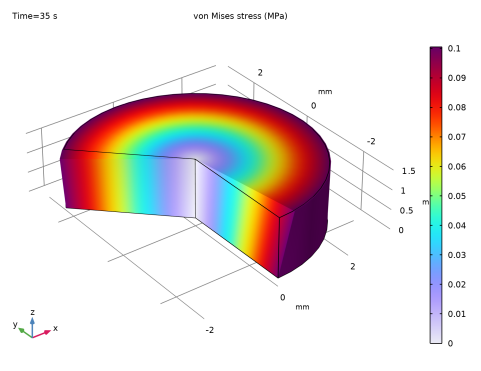
Select the Include circumferential displacement checkbox.
3
Locate the Structural Transient Behavior section. From the list, choose Quasistatic.
Linear Elastic Material 1
1
In the Model Builder window, under Component 1: Torsion Test (comp1) > Solid Mechanics (solid) click Linear Elastic Material 1.
2
In the Settings window for Linear Elastic Material, locate the Linear Elastic Material section.
3
From the Specify list, choose Lamé parameters.
Viscoelasticity, Deviatoric
1
In the Physics toolbar, click  Attributes and choose Viscoelasticity.
2
In the Settings window for Viscoelasticity, type Viscoelasticity, Deviatoric in the Label text field.
3
Locate the Viscoelasticity Model section. In the table, enter the following settings:
4
5
6
7
Linear Elastic Material 1
In the Model Builder window, click Linear Elastic Material 1.
Viscoelasticity, Volumetric
1
In the Physics toolbar, click  Attributes and choose Viscoelasticity.
2
In the Settings window for Viscoelasticity, type Viscoelasticity, Volumetric in the Label text field.
3
Locate the Viscoelasticity Model section. From the Viscoelastic strains list, choose Volumetric.
4
Fixed Constraint 1
1
In the Physics toolbar, click  Boundaries and choose Fixed Constraint.
2
Prescribed Displacement 1
1
In the Physics toolbar, click  Boundaries and choose Prescribed Displacement.
2
3
In the Settings window for Prescribed Displacement, locate the Prescribed Displacement section.
4
From the Displacement in phi direction list, choose Prescribed.
5
In the u0phi text field, type theta*R*step1(t[1/s]).
Global Definitions
Having defined the physics, now fill in the empty expressions in the global Materials node.
Solid Phase (mat1)
1
In the Model Builder window, under Global Definitions > Materials click Solid Phase (mat1).
2
In the Settings window for Material, locate the Material Contents section.
3
Mesh 1
1
In the Model Builder window, under Component 1: Torsion Test (comp1) click Mesh 1.
2
In the Settings window for Mesh, locate the Physics-Controlled Mesh section.
3
From the Element size list, choose Finer.
4
Click  Build All.
Study 1: Torsion Test
1
In the Model Builder window, click Study 1.
2
In the Settings window for Study, type Study 1: Torsion Test in the Label text field.
3
Locate the Study Settings section. Clear the Generate default plots checkbox.
Step 1: Time Dependent
1
In the Model Builder window, under Study 1: Torsion Test click Step 1: Time Dependent.
2
In the Settings window for Time Dependent, locate the Study Settings section.
3
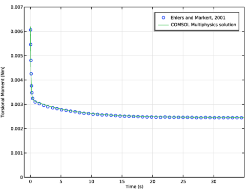
In the Output times text field, type range(0, 0.1, 1) range(1, 1, 35) to resolve the step function properly.
4
In the Study toolbar, click  Compute.
Result Templates
To compare the results with Figure 3, add a Stress, 3D (solid) plot.
1
In the Home toolbar, click  Result Templates to open the Result Templates window.
2
Go to the Result Templates window.
3
In the tree, select Study 1: Torsion Test/Solution 1 (sol1) > Solid Mechanics > Stress, 3D (solid).
4
Click the Add Result Template button in the window toolbar.
5
In the Home toolbar, click  Result Templates to close the Result Templates window.
Results
Surface 1
1
In the Model Builder window, expand the Results > Stress, 3D (solid) node, then click Surface 1.
2
In the Settings window for Surface, locate the Expression section.
3
From the Unit list, choose MPa.
4
In the Stress, 3D (solid) toolbar, click  Plot.
Definitions
To create Figure 4, define a variable for the torsional moment by integrating the reaction moment solid.RMz over the surface boundary. Remember to update the solution so that the newly defined variable is calculated.
Integration 1 (intop1)
1
In the Definitions toolbar, click  Nonlocal Couplings and choose Integration.
2
In the Settings window for Integration, locate the Source Selection section.
3
From the Geometric entity level list, choose Boundary.
4
5
Locate the Advanced section. From the Method list, choose Summation over nodes.
Variables 1
1
In the Model Builder window, right-click Definitions and choose Variables.
2
In the Settings window for Variables, locate the Variables section.
3
Study 1: Torsion Test
In the Study toolbar, click  Update Solution.
Results
Read in the reference data from Ref. 1 for comparison.
Torsion Data, Ehlers and Markert (2001)
1
In the Results toolbar, click  Table.
2
In the Settings window for Table, type Torsion Data, Ehlers and Markert (2001) in the Label text field.
3
Locate the Data section. Click  Import.
4
Torsion Data, Ehlers and Markert (2001)
1
Go to the Torsion Data, Ehlers and Markert (2001) window.
2
Click the Table Graph button in the window toolbar to plot the reference data in a table plot.
Results
Torsional Moment
1
In the Model Builder window, under Results click 1D Plot Group 2.
2
In the Settings window for 1D Plot Group, type Torsional Moment in the Label text field.
Table Graph 1
1
In the Model Builder window, click Table Graph 1.
2
In the Settings window for Table Graph, locate the Coloring and Style section.
3
Find the Line style subsection. From the Line list, choose None.
4
Find the Line markers subsection. From the Marker list, choose Circle.
5
Click to expand the Legends section. Select the Show legends checkbox.
6
From the Legends list, choose Manual.
7
Global 1
1
In the Model Builder window, right-click Torsional Moment and choose Global.
2
In the Settings window for Global, locate the Data section.
3
From the Dataset list, choose Study 1: Torsion Test/Solution 1 (sol1).
4
Click Add Expression in the upper-right corner of the y-Axis Data section. From the menu, choose Component 1: Torsion Test (comp1) > Definitions > Variables > Tm - Torsional moment - N·m.
5
Click to expand the Legends section. From the Legends list, choose Manual.
6
Torsional Moment
1
In the Model Builder window, click Torsional Moment.
2
In the Settings window for 1D Plot Group, locate the Axis section.
3
Select the Manual axis limits checkbox.
4
In the x minimum text field, type -1.
5
In the x maximum text field, type 35.
6
In the y minimum text field, type 0.
7
In the y maximum text field, type 0.007.
8
Click to expand the Title section. From the Title type list, choose None.
9
Locate the Plot Settings section. Select the x-axis label checkbox.
10
Select the y-axis label checkbox. In the associated text field, type Torsional Moment (Nm).
11
Locate the Grid section. Select the Manual spacing checkbox.
12
In the x spacing text field, type 5.
13
In the y spacing text field, type 0.001.
14
In the Torsional Moment toolbar, click  Plot.
Root
Now set up the indentation test. For this purpose, add a second model component.
Add Component
In the Model Builder window, right-click the root node and choose Add Component > 2D Axisymmetric.
Component 2: Indentation Test
In the Settings window for Component, type Component 2: Indentation Test in the Label text field.
Add Physics
1
In the Home toolbar, click  Add Physics to open the Add Physics window.
2
Go to the Add Physics window.
3
In the tree, select Structural Mechanics > Poroelasticity > Poroelasticity, Solid.
4
Click the Add to Component 2: Indentation Test button in the window toolbar.
5
In the Home toolbar, click  Add Physics to close the Add Physics window.
Geometry 2
1
In the Settings window for Geometry, locate the Units section.
2
From the Length unit list, choose mm.
Rectangle 1 (r1)
1
In the Geometry toolbar, click  Rectangle.
2
In the Settings window for Rectangle, locate the Size and Shape section.
3
In the Width text field, type radius_ind.
4
In the Height text field, type height_ind.
5
Click  Build Selected.
Rectangle 2 (r2)
1
In the Geometry toolbar, click  Rectangle.
2
In the Settings window for Rectangle, locate the Size and Shape section.
3
In the Width text field, type 2*r_ind.
4
In the Height text field, type r_ind.
5
Locate the Position section. In the z text field, type height_ind-r_ind.
6
Click  Build Selected.
7
Click the  Zoom Extents button in the Graphics toolbar.
Partition Edges 1 (pare1)
1
In the Geometry toolbar, click  Booleans and Partitions and choose Partition Edges.
2
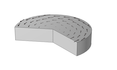
On the object r2, select Boundary 3 only.
3
In the Settings window for Partition Edges, click  Build Selected.
Form Union (fin)
1
In the Model Builder window, click Form Union (fin).
2
In the Settings window for Form Union/Assembly, click  Build Selected.
Mesh Control Domains 1 (mcd1)
1
In the Geometry toolbar, click  Virtual Operations and choose Mesh Control Domains.
2
On the object fin, select Domain 2 only.
3
In the Settings window for Mesh Control Domains, click  Build Selected.
4
In the Geometry toolbar, click  Build All.
Materials
Porous Material 1 (pmat1)
1
In the Model Builder window, under Component 2: Indentation Test (comp2) right-click Materials and choose More Materials > Porous Material.
2
In the Settings window for Porous Material, locate the Phase-Specific Properties section.
3
Click  Add Required Phase Nodes.
Solid 1 (pmat1.solid1)
In the Model Builder window, right-click Porous Material 1 (pmat1) and choose Solid.
The Linear Elastic Material properties in Component 2 are the same as in Component 1, so you can just copy the Viscoelasticity subnodes from there.
Solid Mechanics (solid)
Viscoelasticity, Deviatoric, Viscoelasticity, Volumetric
Right-click and choose Copy.
Solid Mechanics 2 (solid2)
Linear Elastic Material 1
1
In the Model Builder window, under Component 2: Indentation Test (comp2) > Solid Mechanics 2 (solid2) click Linear Elastic Material 1.
2
In the Settings window for Linear Elastic Material, locate the Linear Elastic Material section.
3
From the Specify list, choose Lamé parameters.
4
Right-click Component 2: Indentation Test (comp2) > Solid Mechanics 2 (solid2) > Linear Elastic Material 1 and choose Paste Multiple Items.
Fixed Constraint 1
1
In the Physics toolbar, click  Boundaries and choose Fixed Constraint.
2
Prescribed Displacement 1
1
In the Physics toolbar, click  Boundaries and choose Prescribed Displacement.
2
3
In the Settings window for Prescribed Displacement, locate the Prescribed Displacement section.
4
From the Displacement in z direction list, choose Prescribed.
5
In the u0z text field, type -disp*rm1(t/t_ind).
Darcy’s Law (dl)
Pressure 1
1
In the Physics toolbar, click  Boundaries and choose Pressure.
2
Multiphysics
Poroelasticity 1 (poro1)
1
In the Model Builder window, under Component 2: Indentation Test (comp2) > Multiphysics click Poroelasticity 1 (poro1).
2
In the Settings window for Poroelasticity, locate the Poroelastic Coupling Properties section.
3
From the Poroelasticity model list, choose Biphasic.
4
From the pref list, choose Reference pressure level (dl).
Materials
Now check the material properties and enter additional material properties where needed.
Fluid 1 (pmat1.fluid1)
1
In the Model Builder window, under Component 2: Indentation Test (comp2) > Materials > Porous Material 1 (pmat1) click Fluid 1 (pmat1.fluid1).
2
In the Settings window for Fluid, locate the Fluid Properties section.
3
From the Material list, choose Fluid Phase (mat2).
Global Definitions
Fluid Phase (mat2)
1
In the Model Builder window, under Global Definitions > Materials click Fluid Phase (mat2).
2
In the Settings window for Material, locate the Material Contents section.
3
Materials
Solid 1 (pmat1.solid1)
1
In the Model Builder window, under Component 2: Indentation Test (comp2) > Materials > Porous Material 1 (pmat1) click Solid 1 (pmat1.solid1).
2
In the Settings window for Solid, locate the Solid Properties section.
3
In the θs text field, type phi_solid_ref.
Porous Material 1 (pmat1)
1
In the Model Builder window, click Porous Material 1 (pmat1).
2
In the Settings window for Porous Material, locate the Homogenized Material section.
3
From the Material list, choose Solid Phase (mat1).
4
Click  Go to Material.
Global Definitions
Solid Phase (mat1)
1
In the Model Builder window, under Global Definitions > Materials click Solid Phase (mat1).
2
In the Settings window for Material, locate the Material Contents section.
3
Definitions (comp2)
Add some necessary variable definitions to calculate the indentation force.
Integration 2 (intop2)
1
In the Model Builder window, expand the Component 2: Indentation Test (comp2) > Definitions node.
2
Right-click Component 2: Indentation Test (comp2) > Definitions and choose Nonlocal Couplings > Integration.
3
In the Settings window for Integration, locate the Source Selection section.
4
From the Geometric entity level list, choose Boundary.
5
6
Locate the Advanced section. From the Method list, choose Summation over nodes.
Variables 2
1
Right-click Definitions and choose Variables.
2
In the Settings window for Variables, locate the Variables section.
3
Mesh 2
Free Triangular 1
In the Mesh toolbar, click  Free Triangular.
Size
1
In the Model Builder window, click Size.
2
In the Settings window for Size, locate the Element Size section.
3
From the Predefined list, choose Finer.
Size 1
1
In the Model Builder window, right-click Free Triangular 1 and choose Size.
2
In the Settings window for Size, locate the Geometric Entity Selection section.
3
From the Geometric entity level list, choose Domain.
4
5
Locate the Element Size section. Click the Custom button.
6
Locate the Element Size Parameters section.
7
Select the Maximum element size checkbox. In the associated text field, type 0.05[mm].
8
Click  Build Selected.
Study 1: Torsion Test
Now that you have added a second component to the model, you have to restrict Study 1 to Component 1 in case you want to run it again. Add a second study to solve for the indentation test in Component 2.
Step 1: Time Dependent
1
In the Model Builder window, under Study 1: Torsion Test click Step 1: Time Dependent.
2
In the Settings window for Time Dependent, locate the Physics and Variables Selection section.
3
In the Solve for column of the table, clear the checkbox for Component 2: Indentation Test (comp2).
Add Study
1
In the Home toolbar, click  Add Study to open the Add Study window.
2
Go to the Add Study window.
3
Find the Studies subsection. In the Select Study tree, select General Studies > Time Dependent.
4
Find the Physics interfaces in study subsection. In the table, clear the Solve checkbox for Solid Mechanics (solid).
5
Click the Add Study button in the window toolbar.
6
In the Home toolbar, click  Add Study to close the Add Study window.
Study 2: Indentation Test
1
In the Settings window for Study, type Study 2: Indentation Test in the Label text field.
2
Locate the Study Settings section. Clear the Generate default plots checkbox.
1
In the Model Builder window, under Study 2: Indentation Test click Step 1: Time Dependent.
2
In the Settings window for Time Dependent, locate the Study Settings section.
3
In the Output times text field, type range(0, 0.25*t_ind, t_ind) 10^{range(log10(1.1*t_ind[1/s]),1/15,log10(t_end[1/s]))} t_end.
Add a parametric study to vary the time interval for the loading ramp function.
Parametric Sweep
1
In the Study toolbar, click  Parametric Sweep.
2
In the Settings window for Parametric Sweep, locate the Study Settings section.
3
4
5
In the Study toolbar, click  Compute.
6
Click the  Zoom Extents button in the Graphics toolbar.
Results
To plot Figure 5, follow the steps below.
Result Templates
1
In the Home toolbar, click  Windows and choose Result Templates.
2
Go to the Result Templates window.
3
In the tree, select Study 2: Indentation Test/Parametric Solutions 1 (5) (sol3) > Darcy’s Law > Pressure (dl).
4
Click the Add Result Template button in the window toolbar.
5
In the Results toolbar, click  Result Templates to close the Result Templates window.
Results
Pore Pressure (dl), Indentation Test
1
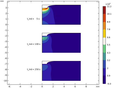
In the Settings window for 2D Plot Group, type Pore Pressure (dl), Indentation Test in the Label text field.
2
Click to collapse the Data section. Click to expand the Data section. From the Parameter value (t_ind (s)) list, choose 5.
3
From the Time (s) list, choose 5.
4
Click to expand the Title section. From the Title type list, choose None.
Surface
1
In the Model Builder window, expand the Pore Pressure (dl), Indentation Test node, then click Surface.
2
In the Settings window for Surface, locate the Coloring and Style section.
3
In the Number of bands text field, type 10.
Deformation 1
Right-click Surface and choose Deformation.
Surface 2
Right-click Surface and choose Duplicate.
Pore Pressure (dl), Indentation Test
1
In the Settings window for 2D Plot Group, click to expand the Plot Array section.
2
From the Array type list, choose Linear.
3
From the Array axis list, choose y.
4
From the Displacement list, choose Absolute.
5
In the Cell displacement text field, type -5.
Surface 2
1
In the Model Builder window, expand the Results > Pore Pressure (dl), Indentation Test > Surface 2 node, then click Surface 2.
2
In the Settings window for Surface, locate the Data section.
3
From the Dataset list, choose Study 2: Indentation Test/Parametric Solutions 1 (5) (sol3).
4
From the Parameter value (t_ind (s)) list, choose 100.
5
From the Time (s) list, choose 100.
6
Click to expand the Inherit Style section. From the Plot list, choose Surface.
7
In the Pore Pressure (dl), Indentation Test toolbar, click  Plot.
Surface 3
1
Right-click Surface 2 and choose Duplicate.
2
In the Settings window for Surface, locate the Data section.
3
From the Parameter value (t_ind (s)) list, choose 250.
4
In the Pore Pressure (dl), Indentation Test toolbar, click  Plot.
5
Click the  Zoom Extents button in the Graphics toolbar.
Pore Pressure (dl), Indentation Test
In the Model Builder window, click Pore Pressure (dl), Indentation Test.
Table Annotation 1
1
In the Pore Pressure (dl), Indentation Test toolbar, click  More Plots and choose Table Annotation.
2
In the Settings window for Table Annotation, locate the Data section.
3
From the Source list, choose Local table.
4
5
Locate the Coloring and Style section. Clear the Show point checkbox.
6
From the Anchor point list, choose Middle left.
7
Click to expand the Plot Array section. Select the Belongs to array checkbox.
8
Select the Manual indexing checkbox.
9
In the Index text field, type 2.
10
In the Pore Pressure (dl), Indentation Test toolbar, click  Plot.
11
Click the  Zoom Extents button in the Graphics toolbar.
Indentation Data, Ehlers and Markert (2001)
Read in the reference data for the indentation test from Ref. 1 to compare the indentation forces.
1
In the Results toolbar, click  Table.
2
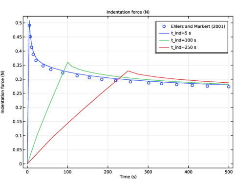
In the Settings window for Table, type Indentation Data, Ehlers and Markert (2001) in the Label text field.
3
Locate the Data section. Click  Import.
4
Indentation Data, Ehlers and Markert (2001)
1
Go to the Indentation Data, Ehlers and Markert (2001) window.
2
Click the Table Graph button in the window toolbar.
Results
Indentation Force
1
In the Model Builder window, under Results click 1D Plot Group 4.
2
In the Settings window for 1D Plot Group, type Indentation Force in the Label text field.
Table Graph 1
1
In the Model Builder window, click Table Graph 1.
2
In the Settings window for Table Graph, locate the Coloring and Style section.
3
Find the Line style subsection. From the Line list, choose None.
4
Find the Line markers subsection. From the Marker list, choose Circle.
5
Locate the Legends section. From the Legends list, choose Manual.
6
Global 1
1
In the Model Builder window, right-click Indentation Force and choose Global.
2
In the Settings window for Global, click Add Expression in the upper-right corner of the y-Axis Data section. From the menu, choose Component 2: Indentation Test (comp2) > Definitions > Variables > comp2.RF - Indentation force - N.
3
Locate the Data section. From the Dataset list, choose Study 2: Indentation Test/Parametric Solutions 1 (4) (sol3).
4
Locate the x-Axis Data section. From the Axis source data list, choose Inner solutions.
5
Click to expand the Coloring and Style section. From the Color list, choose Cycle (reset).
6
In the Indentation Force toolbar, click  Plot.
Table Graph 1
1
In the Model Builder window, click Table Graph 1.
2
In the Settings window for Table Graph, locate the Legends section.
3
Select the Show legends checkbox.
Indentation Force
1
In the Model Builder window, click Indentation Force.
2
In the Settings window for 1D Plot Group, locate the Plot Settings section.
3
Select the y-axis label checkbox.
4
Select the x-axis label checkbox.
5
In the y-axis label text field, type Indentation force (N).
Global 1
1
In the Model Builder window, click Global 1.
2
In the Settings window for Global, locate the Legends section.
3
From the Legends list, choose Manual.
4
5
In the Indentation Force toolbar, click  Plot and compare with Figure 6.