
|
|
|


|
-2.6376·105 Pa
|
||
|
1
|
|
2
|
|
3
|
Click Add.
|
|
4
|
Click
|
|
5
|
|
6
|
Click
|
|
1
|
|
2
|
|
3
|
Locate the Parameters section. In the table, enter the following settings:
|
|
1
|
|
2
|
|
3
|
Locate the Parameters section. In the table, enter the following settings:
|
|
1
|
|
2
|
|
3
|
Locate the Parameters section. In the table, enter the following settings:
|
|
1
|
|
2
|
|
4
|
|
5
|
In the Argument table, enter the following settings:
|
|
1
|
In the Model Builder window, expand the Component 1 (comp1) > Geometry 1 node, then click Geometry 1.
|
|
2
|
|
3
|
|
1
|
|
2
|
|
3
|
|
4
|
|
1
|
|
2
|
|
3
|
|
4
|
|
5
|
|
1
|
|
2
|
On the object r2, select Boundary 3 only.
|
|
3
|
|
5
|
|
1
|
|
2
|
|
3
|
|
4
|
Clear the Create pairs checkbox.
|
|
5
|
|
1
|
|
2
|
|
3
|
|
1
|
|
3
|
|
4
|
Click to select the
|
|
1
|
|
2
|
|
3
|
|
5
|
|
6
|
Browse to the model’s Application Libraries folder and double-click the file hydrogel_swelling_variables.txt.
|
|
1
|
|
2
|
|
3
|
|
1
|
|
1
|
|
3
|
|
4
|
|
5
|
|
6
|
Click to expand the Advanced section. In the Eeq text field, type 3*G. When simulating contact, the equivalent Young’s modulus is used to estimate the contact pressure. For soft materials like gels, the default value is too high, leading to an ill-conditioned problem.
|
|
1
|
|
2
|
|
3
|
|
4
|
|
1
|
|
1
|
|
3
|
|
4
|
|
5
|
|
1
|
In the Model Builder window, under Component 1 (comp1) > Darcy’s Law (dl) > Porous Medium 1 click Fluid 1.
|
|
2
|
|
3
|
|
4
|
|
5
|
|
1
|
|
2
|
|
3
|
|
4
|
|
5
|
Specify the κ matrix as
|
|
1
|
|
2
|
|
3
|
|
1
|
|
2
|
|
3
|
Select the Disconnect pair checkbox.
|
|
1
|
|
2
|
|
4
|
|
1
|
|
2
|
|
3
|
|
1
|
In the Model Builder window, under Component 1 (comp1) > Multiphysics click Poroelasticity 1 (poro1).
|
|
2
|
|
3
|
|
4
|
|
1
|
|
2
|
|
3
|
|
1
|
|
3
|
|
4
|
|
1
|
|
3
|
|
4
|
|
1
|
|
2
|
|
3
|
|
1
|
|
3
|
|
4
|
|
1
|
|
3
|
|
4
|
|
5
|
Click
|
|
1
|
|
2
|
|
3
|
|
1
|
|
2
|
|
3
|
Click
|
|
1
|
|
2
|
|
3
|
|
1
|
|
2
|
Expand the Solution 1 (sol1) node.
|
|
3
|
In the Model Builder window, expand the Inhomogeneous Swelling > Solver Configurations > Solution 1 (sol1) > Dependent Variables 1 node, then click Pressure (comp1.mu).
|
|
4
|
|
5
|
|
6
|
|
7
|
|
8
|
|
9
|
|
10
|
|
11
|
|
12
|
Clear the Interpolate solution at end time checkbox.
|
|
13
|
In the Model Builder window, expand the Inhomogeneous Swelling > Solver Configurations > Solution 1 (sol1) > Time-Dependent Solver 1 node, then click Direct.
|
|
14
|
|
15
|
|
16
|
|
17
|
|
18
|
|
19
|
|
20
|
|
21
|
|
1
|
|
2
|
Go to the Result Templates window.
|
|
3
|
In the tree, select Inhomogeneous Swelling/Parametric Solutions 1 (sol2) > Solid Mechanics > Stress (solid).
|
|
4
|
Click the Add Result Template button in the window toolbar.
|
|
5
|
|
1
|
|
2
|
|
3
|
|
4
|
|
5
|
Clear the Plot dataset edges checkbox.
|
|
1
|
|
2
|
|
3
|
|
4
|
Locate the Data section. From the Dataset list, choose Inhomogeneous Swelling/Parametric Solutions 1 (sol2).
|
|
5
|
|
6
|
|
7
|
|
1
|
|
2
|
|
3
|
|
4
|
|
5
|
|
6
|
|
1
|
|
2
|
|
3
|
|
1
|
|
2
|
|
3
|
|
1
|
|
2
|
|
3
|
|
1
|
|
2
|
|
3
|
|
1
|
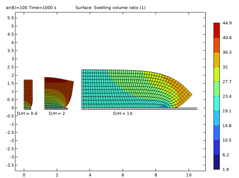
In the Model Builder window, under Results > Swelling Ratio, Ctrl-click to select Surface 2 and Mesh 2.
|
|
2
|
Right-click and choose Duplicate.
|
|
1
|
|
2
|
|
1
|
|
2
|
|
3
|
|
1
|
|
2
|
|
3
|
|
1
|
|
2
|
|
3
|
|
1
|
|
2
|
|
3
|
|
5
|
|
6
|
|
7
|
|
8
|
|
1
|
|
2
|
|
3
|
Locate the Data section. From the Dataset list, choose Inhomogeneous Swelling/Parametric Solutions 1 (sol2).
|
|
4
|
|
5
|
|
6
|
|
7
|
Locate the Plot Settings section.
|
|
8
|
|
9
|
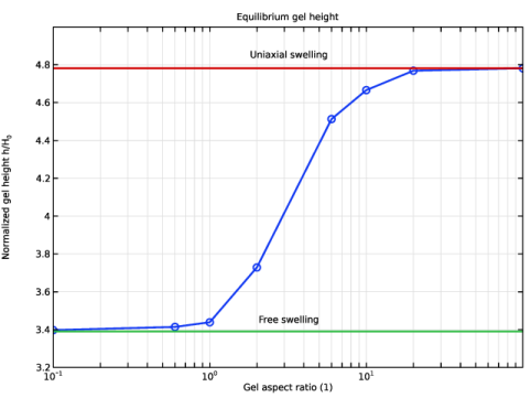
Select the y-axis label checkbox. In the associated text field, type Normalized gel height h/H<sub>0</sub>.
|
|
10
|
|
11
|
|
12
|
|
13
|
|
14
|
|
15
|
Select the x-axis log scale checkbox.
|
|
16
|
|
17
|
|
18
|
|
1
|
|
3
|
|
4
|
|
5
|
|
6
|
|
7
|
|
1
|
|
2
|
Go to the Add Physics window.
|
|
3
|
|
4
|
Click the Add to Component 1 button in the window toolbar.
|
|
5
|
|
1
|
|
3
|
|
4
|
In the Source term quantity table, enter the following settings:
|
|
1
|
|
2
|
Go to the Add Study window.
|
|
3
|
|
4
|
Click the Add Study button in the window toolbar.
|
|
5
|
|
1
|
|
2
|
|
1
|
|
2
|
|
3
|
Select the Modify model configuration for study step checkbox.
|
|
4
|
|
5
|
Click
|
|
6
|
In the tree, select Component 1 (comp1) > Solid Mechanics (solid), Controls spatial frame and Component 1 (comp1) > Darcy’s Law (dl).
|
|
7
|
Click
|
|
8
|
|
9
|
Click
|
|
10
|
Click to expand the Mesh Selection section. In the table, enter the following settings:
|
|
11
|
|
1
|
|
2
|
In the Settings window for Evaluation Group, type Homogeneous Swelling Stretches in the Label text field.
|
|
3
|
|
1
|
|
2
|
|
1
|
|
2
|
|
4
|
|
5
|
|
1
|
|
2
|
|
3
|
|
5
|
|
6
|
|
7
|
|
1
|
|
2
|
|
3
|
Locate the Parameters section. In the table, enter the following settings:
|
|
1
|
|
2
|
|
3
|
Locate the Parameters section. In the table, enter the following settings:
|
|
1
|
|
2
|
|
3
|
|
4
|
|
1
|
|
3
|
|
4
|
|
1
|
|
1
|
|
2
|
|
4
|
|
1
|
|
2
|
|
3
|
|
1
|
|
3
|
|
4
|
|
1
|
|
3
|
|
4
|
|
1
|
|
2
|
|
3
|
|
1
|
|
3
|
|
4
|
|
5
|
Click
|
|
1
|
|
2
|
Go to the Add Study window.
|
|
3
|
|
4
|
Click the Add Study button in the window toolbar.
|
|
5
|
|
1
|
|
2
|
Clear the Generate default plots checkbox.
|
|
3
|
|
1
|
|
2
|
|
3
|
|
4
|
Click
|
|
1
|
|
2
|
|
3
|
|
4
|
Locate the Physics and Variables Selection section. Select the Modify model configuration for study step checkbox.
|
|
5
|
|
6
|
Click
|
|
7
|
In the tree, select Component 1 (comp1) > Darcy’s Law (dl) > Contact (Swelling) and Component 1 (comp1) > Darcy’s Law (dl) > Free Flow (Swelling).
|
|
8
|
Click
|
|
9
|
|
10
|
Click
|
|
1
|
|
2
|
Expand the Solution 12 (sol12) node.
|
|
3
|
In the Model Builder window, expand the Uniaxial Consolidation > Solver Configurations > Solution 12 (sol12) > Dependent Variables 1 node, then click Pressure (comp1.mu).
|
|
4
|
|
5
|
|
6
|
|
7
|
|
8
|
|
9
|
|
10
|
|
11
|
|
12
|
|
13
|
Select the Initial step checkbox.
|
|
14
|
In the Model Builder window, expand the Uniaxial Consolidation > Solver Configurations > Solution 12 (sol12) > Time-Dependent Solver 1 node, then click Direct.
|
|
15
|
|
16
|
|
17
|
|
18
|
|
19
|
|
20
|
|
21
|
|
1
|
|
2
|
|
3
|
|
1
|
|
2
|
Go to the Result Templates window.
|
|
3
|
|
4
|
Click the Add Result Template button in the window toolbar.
|
|
5
|
|
1
|
|
2
|
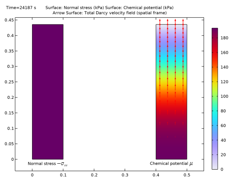
In the Settings window for 2D Plot Group, type Stress and Chemical Potential in the Label text field.
|
|
3
|
|
4
|
|
5
|
|
6
|
|
7
|
|
1
|
|
2
|
|
3
|
|
4
|
|
5
|
|
1
|
|
2
|
|
3
|
|
4
|
|
5
|
|
1
|
|
2
|
|
3
|
|
4
|
|
5
|
Locate the Arrow Positioning section. Find the R grid points subsection. In the Points text field, type 4.
|
|
6
|
|
7
|
|
8
|
Clear the Arrow scale factor checkbox.
|
|
9
|
Clear the Color checkbox.
|
|
10
|
Clear the Color and data range checkbox.
|
|
11
|
|
12
|
|
1
|
|
2
|
|
3
|
|
5
|
Select the LaTeX markup checkbox.
|
|
6
|
|
7
|
|
1
|
|
2
|
|
3
|
|
4
|
In the Title text area, type
|
|
5
|
|
6
|
|
1
|
|
2
|
|
3
|
|
4
|
Locate the Plot Settings section.
|
|
5
|
|
6
|
|
7
|
|
8
|
|
9
|
|
10
|
|
11
|
|
12
|
|
13
|
|
14
|
|
1
|
|
3
|
|
4
|
|
5
|
|
6
|
|
7
|
|
8
|
|
1
|
|
2
|
|
3
|
|
5
|
Select the LaTeX markup checkbox.
|
|
6
|
|
7
|
|
8
|
|
1
|
|
2
|
In the Settings window for Table, type Reference Data, Hong and others (2008), t=2 in the Label text field.
|
|
3
|
|
4
|
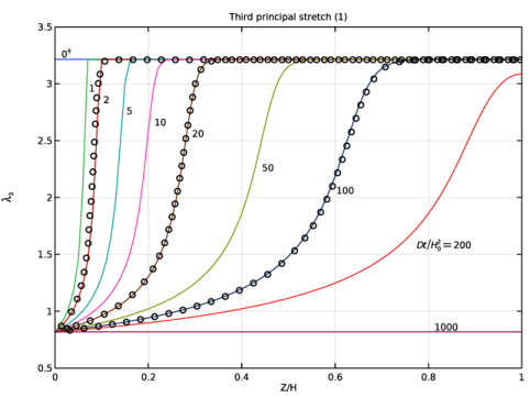
Browse to the model’s Application Libraries folder and double-click the file hydrogel_swelling_uniaxial_t2.txt.
|
|
1
|
|
2
|
In the Settings window for Table, type Reference Data, Hong and others (2008), t=20 in the Label text field.
|
|
3
|
|
4
|
Browse to the model’s Application Libraries folder and double-click the file hydrogel_swelling_uniaxial_t20.txt.
|
|
1
|
|
2
|
In the Settings window for Table, type Reference Data, Hong and others (2008), t=100 in the Label text field.
|
|
3
|
|
4
|
Browse to the model’s Application Libraries folder and double-click the file hydrogel_swelling_uniaxial_t100.txt.
|
|
1
|
|
2
|
|
3
|
|
4
|
|
5
|
|
6
|
|
1
|
|
2
|
|
3
|
|
4
|
|
1
|
|
2
|
In the Settings window for Table Graph, type Reference Data, Hong and others (2008), t=100 in the Label text field.
|
|
3
|
|
4
|
|
1
|
|
2
|
|
3
|
Select the Modify model configuration for study step checkbox.
|
|
4
|
|
5
|
Click
|
|
6
|
In the tree, select Component 1 (comp1) > Solid Mechanics (solid), Controls spatial frame > Boundary Load 1 and Component 1 (comp1) > Solid Mechanics (solid), Controls spatial frame > Roller 1.
|
|
7
|
Click
|
|
8
|
|
9
|
Click
|
