
|
|
|

|
1
|
|
2
|
In the Select Physics tree, select Fluid Flow > Nonisothermal Flow > Rotating Machinery, Nonisothermal Flow > Laminar Flow.
|
|
3
|
Click Add.
|
|
4
|
Click
|
|
5
|
|
6
|
Click
|
|
1
|
|
2
|
Browse to the model’s Application Libraries folder and double-click the file pasta_extrusion_geom_sequence.mph.
|
|
3
|
|
4
|
|
5
|
|
6
|
Clear the Automatic detection of small details checkbox.
|
|
7
|
|
1
|
|
2
|
|
3
|
|
4
|
Click to expand the Override section. Locate the Rotation section. In the f text field, type 20[RPM].
|
|
5
|
|
1
|
In the Model Builder window, under Component 1 (comp1) > Laminar Flow (spf) click Fluid Properties 1.
|
|
2
|
|
3
|
|
1
|
In the Model Builder window, under Component 1 (comp1) right-click Materials and choose Blank Material.
|
|
2
|
|
1
|
|
2
|
Right-click Component 1 (comp1) > Materials > Material 1 (mat1) > Power law (PowerLaw) and choose Functions > Interpolation.
|
|
3
|
|
4
|
|
6
|
|
7
|
In the Argument table, enter the following settings:
|
|
1
|
|
2
|
|
3
|
|
5
|
|
1
|
In the Model Builder window, under Component 1 (comp1) > Materials > Material 1 (mat1) click Power law (PowerLaw).
|
|
2
|
|
4
|
|
5
|
|
6
|
In the Model Builder window, collapse the Component 1 (comp1) > Materials > Pasta 30% Hydration (mat1) > Power law (PowerLaw) node.
|
|
1
|
|
2
|
|
3
|
|
4
|
Select the Neglect inertial term (Stokes flow) checkbox.
|
|
1
|
In the Model Builder window, under Component 1 (comp1) > Creeping Flow (spf) click Fluid Properties 1.
|
|
2
|
|
1
|
|
2
|
|
3
|
|
4
|
|
1
|
|
2
|
|
3
|
|
1
|
|
2
|
|
3
|
|
4
|
Click to expand the Wall Movement section. From the Translational velocity list, choose Zero (Fixed wall).
|
|
1
|
|
2
|
|
3
|
|
1
|
|
2
|
|
3
|
|
4
|
|
1
|
|
2
|
|
3
|
|
4
|
|
5
|
|
6
|
|
1
|
|
2
|
|
3
|
|
4
|
Click
|
|
1
|
|
2
|
|
3
|
Clear the Generate default plots checkbox.
|
|
4
|
|
1
|
|
2
|
Go to the Result Templates window.
|
|
3
|
|
4
|
Click the Add Result Template button in the window toolbar.
|
|
1
|
|
2
|
|
3
|
|
4
|
|
5
|
|
1
|
|
2
|
|
3
|
|
4
|
|
1
|
|
2
|
|
3
|
|
1
|
|
2
|
|
3
|
|
4
|
|
5
|
|
6
|
|
7
|
|
1
|
|
2
|
|
1
|
|
2
|
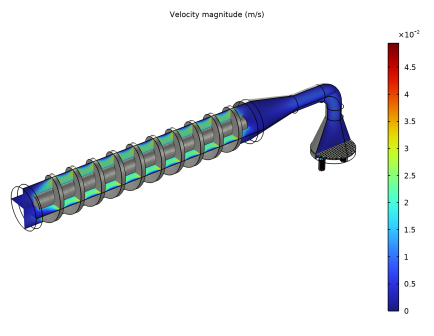
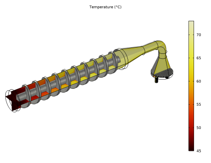
In the Settings window for Multislice, click Replace Expression in the upper-right corner of the Expression section. From the menu, choose Component 1 (comp1) > Heat Transfer in Fluids > Temperature > T - Temperature - K.
|
|
3
|
|
4
|
|
5
|
|
1
|
|
2
|
|
1
|
|
2
|
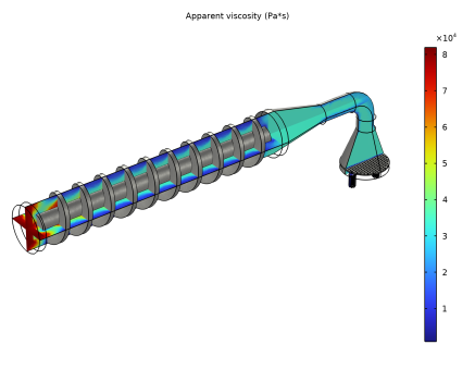
In the Settings window for Multislice, click Replace Expression in the upper-right corner of the Expression section. From the menu, choose Component 1 (comp1) > Creeping Flow > Material properties > spf.mu_app - Apparent viscosity - Pa·s.
|
|
3
|
|
1
|
|
2
|
|
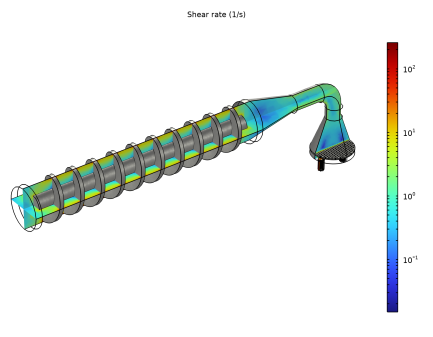
1
|
In the Model Builder window, expand the Viscosity 1 node, then click Results > Shear Rate > Multislice 1.
|
|
2
|
In the Settings window for Multislice, click Replace Expression in the upper-right corner of the Expression section. From the menu, choose Component 1 (comp1) > Creeping Flow > Velocity and pressure > spf.sr - Shear rate - 1/s.
|
|
3
|
|
4
|