|
|
|

|
|
|||
|
•
|
If a species is set From mass constraint it does not need any Inlet and Outflow subfeature since its mass fraction is computed so that the mass in the system is conserved. There are no dependent variables being solved for the mass constraint species and as such does not need the boundary conditions set by the subfeatures.
|
|
•
|
If the feed into the system contains another species (the present model does not have) one of these species should be set as mass constraint and the other should use an Inlet subfeature that specifies the appropriate proportion. Consider as an example of a feed of Ar/O2 at 60/40 mole fraction. If Ar is set as mass constrain than O2 should have an Inlet subfeature with a mole fraction of 0.4.
|
|
•
|
If the species in created inside the reactor (as are Ar+ and Ars) no Inlet subfeature should be added.
|
|
•
|
If the species flows out of the system (as are Ar+ and Ars) an Outflow subfeature should be added.
|
|
1
|
|
2
|
|
3
|
Click Add.
|
|
4
|
Click
|
|
5
|
|
6
|
Click
|
|
1
|
|
2
|
In the Show More Options dialog, in the tree, select the checkbox for the node Physics > Advanced Physics Options.
|
|
3
|
|
4
|
Click OK.
|
|
1
|
|
2
|
|
3
|
Click
|
|
4
|
Browse to the model’s Application Libraries folder and double-click the file thermal_plasma.mphbin.
|
|
5
|
Click
|
|
1
|
|
2
|
|
1
|
|
3
|
|
1
|
|
2
|
|
3
|
|
5
|
|
1
|
|
2
|
|
3
|
|
5
|
|
1
|
|
2
|
|
3
|
|
5
|
|
1
|
|
2
|
|
3
|
|
1
|
|
2
|
|
3
|
Click
|
|
5
|
Click
|
|
6
|
|
7
|
|
8
|
Select the Use reduced electron transport properties checkbox.
|
|
1
|
|
2
|
|
3
|
|
4
|
|
1
|
|
2
|
|
3
|
|
4
|
|
1
|
|
2
|
|
3
|
|
1
|
|
2
|
|
3
|
|
4
|
|
1
|
|
2
|
|
3
|
|
4
|
|
1
|
|
2
|
|
3
|
|
1
|
|
2
|
|
3
|
|
4
|
|
1
|
|
2
|
|
3
|
Select the From mass constraint checkbox.
|
|
4
|
|
1
|
|
2
|
|
3
|
|
4
|
|
5
|
|
1
|
|
2
|
|
3
|
Select the Initial value from electroneutrality constraint checkbox.
|
|
4
|
|
5
|
|
1
|
|
2
|
|
3
|
|
1
|
|
2
|
|
3
|
|
4
|
|
1
|
|
3
|
|
4
|
|
5
|
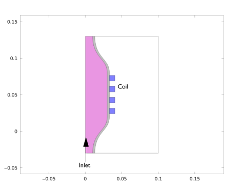
Select the Coil group checkbox.
|
|
6
|
|
1
|
|
2
|
|
3
|
|
4
|
|
5
|
|
7
|
|
1
|
|
3
|
|
4
|
From the list, choose Mass flow.
|
|
5
|
|
6
|
|
1
|
|
1
|
|
2
|
|
3
|
Click
|
|
1
|
In the Model Builder window, under Component 1 (comp1) > Heat Transfer in Fluids (ht) click Initial Values 1.
|
|
2
|
|
3
|
|
1
|
|
3
|
|
4
|
|
1
|
|
1
|
In the Model Builder window, under Component 1 (comp1) right-click Materials and choose Blank Material.
|
|
3
|
|
5
|
|
1
|
|
3
|
|
5
|
|
1
|
|
3
|
|
5
|
|
1
|
|
2
|
|
3
|
|
1
|
|
1
|
|
2
|
|
3
|
|
4
|
Click to expand the Element Size Parameters section. Locate the Element Size section. Click the Custom button.
|
|
5
|
Locate the Element Size Parameters section.
|
|
6
|
|
1
|
|
2
|
|
3
|
|
1
|
|
2
|
|
3
|
|
1
|
|
2
|
|
3
|
|
1
|
|
2
|
|
3
|
|
4
|
|
5
|
|
1
|
|
2
|
|
3
|
|
1
|
|
2
|
|
3
|
|
4
|
|
5
|
|
6
|
|
7
|
|
8
|
Select the Symmetric distribution checkbox.
|
|
1
|
|
2
|
|
1
|
|
2
|
|
3
|
|
4
|
Click
|
|
5
|
|
6
|
|
7
|
|
8
|
|
9
|
|
10
|
Click Add.
|
|
11
|
|
12
|
|
13
|
|
1
|
|
2
|
|
1
|
|
2
|
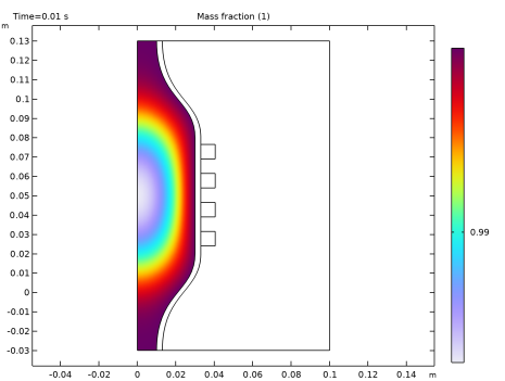
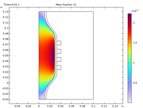
In the Settings window for Surface, click Replace Expression in the upper-right corner of the Expression section. From the menu, choose Component 1 (comp1) > Plasma > Mass fractions > plas.wAr - Mass fraction - 1.
|
|
3
|
|
1
|
|
2
|
|
1
|
|
2
|
In the Settings window for Surface, click Replace Expression in the upper-right corner of the Expression section. From the menu, choose Component 1 (comp1) > Plasma > Mass fractions > plas.wArs - Mass fraction - 1.
|
|
3
|