
|
|
|


|
SFx
|
||
|
Fx
|
||
|
1
|
|
2
|
|
3
|
Click Add.
|
|
4
|
Click
|
|
5
|
|
6
|
Click
|
|
1
|
|
2
|
|
1
|
|
2
|
|
3
|
|
1
|
|
2
|
|
3
|
|
4
|
|
5
|
Click
|
|
1
|
|
2
|
|
3
|
|
4
|
|
5
|
|
6
|
Click to expand the Heavy Species Energy Balance section. Select the Include heavy species energy conservation equation checkbox.
|
|
1
|
|
2
|
|
3
|
|
4
|
|
5
|
|
6
|
|
7
|
|
8
|
|
9
|
|
10
|
|
11
|
|
1
|
|
2
|
|
3
|
Click
|
|
4
|
Browse to the model’s Application Libraries folder and double-click the file SF6_Ar_plasma_chemistry.txt.
|
|
5
|
Click
|
|
1
|
In the Model Builder window, expand the Component 1 (comp1) > Plasma (plas) > Group - Species node, then click Species: SF6.
|
|
2
|
|
3
|
Select the From mass constraint checkbox.
|
|
4
|
|
1
|
|
2
|
|
3
|
|
1
|
|
2
|
|
3
|
|
1
|
|
2
|
|
3
|
|
1
|
|
2
|
|
3
|
|
1
|
|
2
|
|
3
|
|
1
|
|
2
|
|
3
|
|
1
|
|
2
|
|
3
|
|
1
|
|
2
|
|
3
|
|
4
|
|
1
|
|
2
|
|
3
|
|
5
|
Click
|
|
1
|
|
2
|
Go to the Add Study window.
|
|
3
|
|
4
|
Click the Add Study button in the window toolbar.
|
|
5
|
|
1
|
|
2
|
|
1
|
|
2
|
|
3
|
Find the Initial values of variables solved for subsection. From the Settings list, choose User controlled.
|
|
4
|
|
5
|
|
6
|
|
7
|
Click
|
|
10
|
Click
|
|
11
|
|
12
|
|
13
|
|
14
|
Click Add.
|
|
15
|
|
1
|
|
2
|
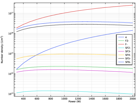
In the Settings window for 1D Plot Group, type Species densities vs. Power - Neutral in the Label text field.
|
|
3
|
|
4
|
|
5
|
Locate the Plot Settings section.
|
|
6
|
|
7
|
Select the y-axis label checkbox. In the associated text field, type Number density (1/m<sup>3</sup>).
|
|
8
|
|
9
|
|
1
|
|
2
|
|
4
|
|
5
|
|
1
|
In the Model Builder window, right-click Species densities vs. Power - Neutral and choose Duplicate.
|
|
2
|
In the Settings window for 1D Plot Group, type Species densities vs. Power - Positive in the Label text field.
|
|
3
|
|
1
|
In the Model Builder window, expand the Species densities vs. Power - Positive node, then click Global 1.
|
|
2
|
|
3
|
Click
|
|
5
|
|
1
|
In the Model Builder window, right-click Species densities vs. Power - Positive and choose Duplicate.
|
|
2
|
In the Settings window for 1D Plot Group, type Species densities vs. Power - Negative in the Label text field.
|
|
3
|
|
1
|
In the Model Builder window, expand the Species densities vs. Power - Negative node, then click Global 1.
|
|
2
|
|
3
|
Click
|
|
5
|
|
1
|
|
2
|
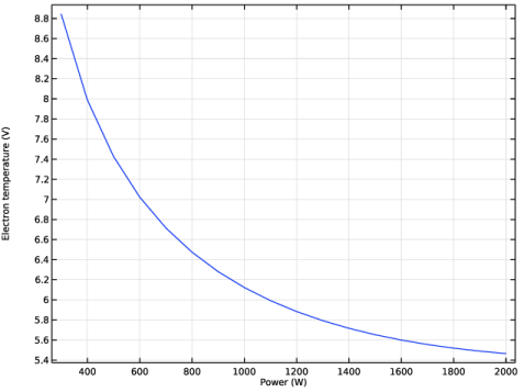
In the Settings window for 1D Plot Group, type Electron Temperature vs. Power in the Label text field.
|
|
3
|
|
4
|
|
5
|
Locate the Plot Settings section.
|
|
6
|
|
7
|
|
1
|
|
2
|
|
4
|
|
1
|
|
2
|
|
3
|
|
4
|
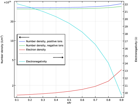
Select the y-axis label checkbox. In the associated text field, type Number density (1/m<sup>3</sup>).
|
|
5
|
Select the Secondary y-axis label checkbox. In the associated text field, type Electronegativity (1).
|
|
6
|
|
7
|
|
1
|
|
2
|
|
3
|
Select the Plot on secondary y-axis checkbox.
|
|
4
|
Locate the y-Axis Data section. In the table, enter the following settings:
|
|
1
|
|
2
|
|
3
|
Click
|
|
5
|
|
6
|
|
1
|
|
2
|
|
1
|
|
2
|
|
3
|
Click
|
|
5
|
|
1
|
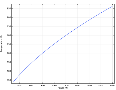
In the Model Builder window, under Results, Ctrl-click to select Species densities vs. Power - Neutral, Species densities vs. Power - Positive, Species densities vs. Power - Negative, Electron Temperature vs. Power, Electronegativity vs. Power, and Gas Temperature vs. Power.
|
|
2
|
Right-click and choose Group.
|
|
1
|
|
2
|
|
1
|
|
2
|
Go to the Add Study window.
|
|
3
|
|
4
|
Click the Add Study button in the window toolbar.
|
|
5
|
|
1
|
|
2
|
|
1
|
|
2
|
|
3
|
Find the Initial values of variables solved for subsection. From the Settings list, choose User controlled.
|
|
4
|
|
5
|
|
6
|
|
7
|
|
8
|
Click
|
|
11
|
Click
|
|
12
|
|
13
|
|
14
|
|
15
|
Click Add.
|
|
16
|
|
1
|
|
2
|
|
1
|
In the Model Builder window, expand the xAr Sweep node, then click Species densities vs. Power - Neutral 1.
|
|
2
|
In the Settings window for 1D Plot Group, type Species densities vs. xAr - Neutral in the Label text field.
|
|
3
|
|
4
|
|
5
|
|
6
|
|
1
|
In the Model Builder window, under Results > xAr Sweep click Species densities vs. Power - Positive 1.
|
|
2
|
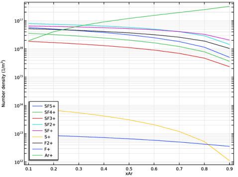
In the Settings window for 1D Plot Group, type Species densities vs. xAr - Positive in the Label text field.
|
|
3
|
|
4
|
|
5
|
|
6
|
|
1
|
In the Model Builder window, under Results > xAr Sweep click Species densities vs. Power - Negative 1.
|
|
2
|
In the Settings window for 1D Plot Group, type Species densities vs. xAr - Negative in the Label text field.
|
|
3
|
|
4
|
|
5
|
|
1
|
|
2
|
In the Settings window for 1D Plot Group, type Electron Temperature vs. xAr in the Label text field.
|
|
3
|
|
4
|
|
5
|
|
1
|
|
2
|
|
3
|
|
4
|
|
5
|
|
6
|
|
1
|
|
2
|
|
3
|
|
4
|
|
5
|
 .
.