COMSOL 6.4 - Microwave Plasma Torch

This tutorial demonstrates how to set up a 3D model of a microwave plasma torch operating with argon at moderate pressures. The model is based on a generic configuration in which the plasma is generated inside a dielectric tube inserted into a rectangular waveguide. A useful reference for this type of plasma reactor is Ref. 1. Microwave power at 2.45 GHz is introduced into the waveguide in the TE01 mode, with the opposite end of the waveguide short-circuited. The dielectric tube is positioned at the location of maximum electromagnetic field intensity. The simulation solves a fully self-consistent set of coupled equations, including plasma transport and heating, Maxwell’s equations, fluid flow, and heat transfer

The model requires the Plasma Module and RF Module.

Model Definition

Electron transport is modeled by solving the continuity equation, the momentum equation under the drift-diffusion approximation, and the mean electron energy equation (for detailed information on electron transport, see Theory for the Drift Diffusion Interface in the Plasma Module User’s Guide)

The source coefficients in the above equations are determined by the plasma chemistry. The electron rate expression is defined as

where νe,j is the stoichiometric coefficient, and the reaction rate is defined as

where kjf is the forward rate constant and kjr is the reversed rate constant. Both the Electron Impact Reaction feature and Reaction feature can contribute to the electron rate expression. However, when using the Reaction feature it is important to note that the associated electron energy gain or loss is not included in the source term of the electron mean energy equation.

The rate constants can be computed from electron impact cross-section data

where γ = (2q/me)1/2 (SI unit: C1/2/kg1/2), me is the electron mass (SI unit: kg), ε is the electron energy (SI unit: V), σ is the electron impact collision cross section (SI unit: m2), and f is the electron energy distribution function.

When Townsend coefficients are used, the reaction rate is defined as

where αj/Nn is the reduced Townsend coefficient for reaction j (SI unit: m2) and Γe is the electron flux as defined above (SI unit: 1/(m2·s)). Townsend coefficients can increase the stability of the numerical scheme when the electron flux is field driven as is the case with DC discharges.

The total electron energy loss or gained is calculated by summing the collisional energy changes from all reactions defined with the Electron Impact Reaction feature as

where Δεj is the energy loss from reaction j (SI unit: V) and F is the Faraday constant (SI unit: C/mol). For excitation and ionization collisions Δεj corresponds to the energy of the excited state being excited/deexcited or ionized, for attachment Δεj is set to zero, and for elastic collisions

where me and mk are the electron and heavy species mass in kg, Te is the electron temperature in eV, and Tgas is the gas temperature in K.

For heavy species, the following equation is solved for the mass fraction of each species (for detailed information on the transport of the nonelectron species, see Theory for the Heavy Species Transport Interface in the Plasma Module User’s Guide):

The electrostatic field is computed using the following equation:

The space charge density ρ is automatically computed based on the plasma chemistry specified in the model using the formula

For detailed information about electrostatics see Theory for the Electrostatics Interface in the Plasma Module User’s Guide.

In a microwave reactor the high frequency electric field is computed in the frequency domain using the following equation:

The electromagnetic wave “sees” a plasma defined by the plasma conductivity in the cold plasma approximation that is set in the multiphysics feature:

where ne is the electron density, q is the electron charge, me is the electron mass, νe is the collision frequency, and ω is the angular frequency. The Joule heating term that is responsible to heat the electrons is set in the multiphysics feature.

plasma chemistry

Argon plasmas feature one of the simplest reaction schemes, with electronically excited states often lumped into single effective levels. At high pressures, three-body reactions become significant, leading to the formation of dimers. The model employs a simplified plasma chemistry similar to that described in Ref. 2, comprising nine volumetric reactions involving electrons (with electron impact cross sections obtained from Ref. 2), atomic and molecular ions, and a lumped level representing the argon 4s excited state.

Table 1: table of collisions and reactions modeled.
reaction	formula	type
1	e+Ar=>e+Ar	Elastic	0
2	e+Ar=>e+Ars	Excitation	11.5
3	e+Ars=>e+Ar	Superelastic	-11.5
4	e+Ar=>2e+Ar+	Ionization	15.8
5	e+Ars=>2e+Ar+	Ionization	4.24
6	e+Ar2+=>Ars+Ar	Excitation	-2.5
7	Ars+Ars=>e+Ar+Ar+	Penning ionization	-
8	Ars=>Ar	Spontaneous emission	-
9	2Ar+Ar+=>Ar+Ar2+	3-body Ar2+ creation	-

In addition to volumetric reactions, the following surface reactions are implemented:

Table 2: table of surface reactions.
reaction	formula	Sticking Coefficient
1	Ars=>Ar	1
2	Ar+=>Ar	1
3	Ar2+=>2Ar	1

Results and Discussion

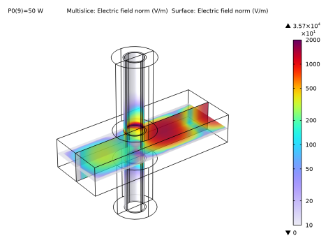
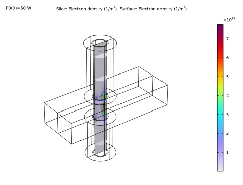
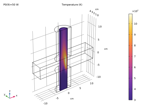
The figures in this section present the simulation results for an argon plasma sustained at 20 Torr with 50 W of input power. Figure 1 displays the spatial distribution of the electric field norm, where the maximum field intensity is observed at the interface between the waveguide and the dielectric tube, proximal to the microwave power injection port. This localized field enhancement corresponds to a region of elevated ionization, where the electron density reaches peak values of the order of 1018 m-3, as shown in Figure 2. At such high plasma densities, energy transfer to neutral argon atoms via electron impact elastic collisions becomes significant, resulting in a neutral gas temperature increase up to 1000 K, as illustrated in Figure 3. Due to the gas inflow at the bottom of the dielectric tube, the gas temperature and number density, and consequently the charged species densities, exhibit asymmetry along the axial (z) direction.

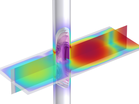
Figure 4 presents the electron density isosurfaces along with the electric field norm in a logarithmic scale. The results clearly demonstrates that the presence of the plasma significantly alters the electromagnetic field distribution, with the electric field amplitude attenuating rapidly upon entering the plasma region due to plasma shielding. Additionally, the electron density exhibits localized maxima near the waveguide-dielectric tube junction, forming an annular distribution pattern. This structure is indicative of enhance ionization near the periphery of the discharge channel.

Figure 1: Electric field norm in the waveguide and at the surface of the dielectric tube for an input power of 50 W.

Figure 2: Electron number density for an input power of 50 W.

Figure 3: Gas temperature for an input power of 50 W.

Figure 4: Electric field norm and electron number density isosurfaces on a logarithmic scale for an input power of 50 W. The electron number density isosurface levels are: 0.05, 0.11, 0.23, 0.5, 1.1, 2.3, and 50 in units of 1018 m-3. The electric field norm has the same scale as in Figure 1.

References

1. M. Baeva, F. Hempel, H. Baiel, T. Trautvetter, R. Foest, and D. Loffhagen, “Two- and three-dimensional simulation analysis of a microwave excited plasma for deposition application: operation with argon at atmospheric pressure,” J. Phys. D: Appl. Phys., vol. 51, p. 385202, 2018.

2. N. Balcon, G.J.M. Hagelaar, and J.P. Boeuf, “Numerical Model of an Argon Atmospheric Pressure RF Discharge,” IEEE Trans. Plasma Sci., vol. 36, p. 2782, 2008.

3. Phelps database, www.lxcat.net, retrieved 2017.

Plasma_Module/Wave-Heated_Discharges/microwave_plasma_torch

Modeling Instructions

From the menu, choose .

New

In the window, click

Model Wizard

In the window, click

In the tree, select > > .

Click .

Click

In the tree, select > .

Click

Geometry 1

In the window, under click .

In the window for , locate the section.

From the list, choose .

Global Definitions

Parameters 1

Import parameters to use in the model.

In the window, under click .

In the window for , locate the section.

Click

Browse to the model’s Application Libraries folder and double-click the file microwave_plasma_torch_parameters.txt.

Next, create a geometry for a microwave plasma torch.

Geometry 1

Block 1 (blk1)

In the toolbar, click

In the window for , locate the section.

In the text field, type WaveguideLength.

In the text field, type WaveguideWidth.

In the text field, type WaveguideHeight.

Locate the section. From the list, choose .

Cylinder 1 (cyl1)

In the toolbar, click

In the window for , locate the section.

In the text field, type RadiusOut.

In the text field, type CylinderHeight*(1+TopCylinderFactor).

Locate the section. In the text field, type CylincerCenter.

In the text field, type -CylinderHeight/2.

Click to expand the section. In the table, enter the following settings:


Layer name	Thickness (cm)
Layer 1	RadiusOut-RadiusIn

Click

Cylinder 2 (cyl2)

In the toolbar, click

In the window for , locate the section.

In the text field, type RadiusOut*2.

In the text field, type (CylinderHeight*(1+2*TopCylinderFactor))/2-WaveguideHeight/2.

Locate the section. In the text field, type CylincerCenter.

In the text field, type WaveguideHeight/2.

Cylinder 3 (cyl3)

Right-click and choose .

In the window for , locate the section.

In the text field, type CylinderHeight/2-WaveguideHeight/2.

Locate the section. In the text field, type -CylinderHeight/2.

Click

Work Plane 1 (wp1)

In the toolbar, click

In the window for , locate the section.

From the list, choose .

Partition Objects 1 (par1)

In the toolbar, click

and choose .

Click in the window and then press Ctrl+A to select all objects.

In the window for , locate the section.

From the list, choose .

Delete Entities 1 (del1)

In the window, right-click and choose .

In the window for , locate the section.

From the list, choose .

On the object , select Domain 1 only.

On the object , select Domains 1, 3, and 5 only.

On the object , select Domain 1 only.

Click

Create explicit selections for later use.

Geometry 1

In the window, collapse the > node.

Definitions

Tube

In the toolbar, click

In the window for , type Tube in the text field.

Select Domains 4–6 and 10–12 only.

Walls

In the toolbar, click

In the window for , type Walls in the text field.

Locate the section. From the list, choose .

Click the

button in the toolbar.

Select Boundaries 24, 27, 30, 35, 38, and 41 only.

Plasma

In the toolbar, click

In the window for , type Plasma in the text field.

Click the

button in the toolbar.

Select Domains 7–9 only.

Specify material properties for use by the different physics interfaces.

Add Material

In the toolbar, click

to open the window.

Go to the window.

In the tree, select > .

Click the button in the window toolbar.

In the tree, select > .

Click the button in the window toolbar.

In the toolbar, click

to close the window.

Materials

Glass (quartz) (mat2)

In the window for , locate the section.

From the list, choose .

In the interface, prepare a simple plasma chemistry for argon and apply boundary conditions for all species being solved. Poisson’s equation is only solved in the plasma domain, and for simplicity the electric potential is set to zero at the dielectric.

On the symmetry plane, make sure that the default boundary conditions — and — are used, and that no surface reaction is applied.

Plasma (plas)

Cross Section Import 1

In the toolbar, click

and choose .

In the window for , locate the section.

Click

Browse to the model’s Application Libraries folder and double-click the file Ar_xsecs.txt.

Click

Electron Impact Reaction 6

In the toolbar, click

and choose .

In the window for , locate the section.

In the text field, type e+Ar2+=>Ars+Ar.

Locate the section. From the list, choose .

In the Δε text field, type -2.5[V].

Locate the section. In the kf text field, type 7e-13[m^3/s]*N_A_const*(300[K]/(plas.Te*11600[K/V]))^0.5.

Reaction 1

In the toolbar, click

and choose .

In the window for , locate the section.

In the text field, type Ars+Ars=>e+Ar+Ar+.

Locate the section. In the kf text field, type 1.2e-15[m^3/s]*N_A_const.

Reaction 2

In the toolbar, click

and choose .

In the window for , locate the section.

In the text field, type Ars=>Ar.

Locate the section. In the kf text field, type 5e5[1/s].

Reaction 3

In the toolbar, click

and choose .

In the window for , locate the section.

In the text field, type Ar+Ar+Ar+=>Ar2++Ar.

Locate the section. In the kf text field, type 2.5e-43[m^6/s]*N_A_const^2.

Species: Ar

In the window, click .

In the window for , locate the section.

Select the checkbox.

Locate the section. From the list, choose .

Species: Ars

In the window, click .

In the window for , locate the section.

From the list, choose .

Click to expand the section. In the Δh text field, type 11.50.

Species: Ar+

In the window, click .

In the window for , locate the section.

From the list, choose .

Locate the section. In the Δh text field, type 15.80.

Species: Ar2+

In the window, click .

In the window for , locate the section.

In the Mw text field, type 0.08[kg/mol].

In the σ text field, type 3.330[angstrom].

In the ε/kb text field, type 136.500[K].

Locate the section. In the alow,1 text field, type 0.02500000E+02.

In the alow,6 text field, type -0.07453750E+04.

In the alow,7 text field, type 0.04366000E+02.

In the ahi,1 text field, type 0.02500000E+02.

In the ahi,6 text field, type -0.07453750E+04.

In the ahi,7 text field, type 0.04366000E+02.

In the Δh text field, type 14.5.

Surface Reaction 1

In the toolbar, click

and choose .

In the window for , locate the section.

In the text field, type Ar+=>Ar.

Locate the section. From the list, choose .

Surface Reaction 2

In the toolbar, click

and choose .

In the window for , locate the section.

In the text field, type Ars=>Ar.

Locate the section. From the list, choose .

Surface Reaction 3

In the toolbar, click

and choose .

In the window for , locate the section.

In the text field, type Ar2+=>2Ar.

Locate the section. From the list, choose .

Plasma Model 1

In the window, click .

In the window for , locate the section.

From the list, choose .

Initial Values 1

In the window, click .

In the window for , locate the section.

In the ne,0 text field, type 1E16[1/m^3].

Wall 1

In the toolbar, click

and choose .

In the window for , locate the section.

From the list, choose .

Outflow 1

In the toolbar, click

and choose .

Select Boundary 33 only.

Ground 1

In the toolbar, click

and choose .

In the window for , locate the section.

From the list, choose .

In the window, click .

In the window for , locate the section.

Click

From the list, choose .

In the interface, set the domain where the physics is to be solved, add an inlet and outlet to the system, and set the symmetry plane.

Laminar Flow (spf)

In the window, under click .

In the window for , locate the section.

From the list, choose .

Locate the section. In the pref text field, type p0.

Inlet 1

In the toolbar, click

and choose .

Select Boundary 26 only.

In the window for , locate the section.

From the list, choose .

Locate the section. From the list, choose .

In the Qsv text field, type Qsv.

Outlet 1

In the toolbar, click

and choose .

Select Boundary 33 only.

Symmetry 1

In the toolbar, click

and choose .

Select Boundaries 25, 28, and 31 only.

Laminar Flow (spf)

In the window, collapse the > node.

Specify the domains where the interface is to be solved, set a constant temperature at the inlet, use a heat flux boundary conditions in the dielectric, and set the symmetry plane.

Heat Transfer in Fluids (ht)

In the window, under click .

In the window for , locate the section.

In the Tref text field, type T0.

Locate the section. From the list, choose .

Select Domains 4–12 only.

Solid 1

In the toolbar, click

and choose .

In the window for , locate the section.

From the list, choose .

Outflow 1

In the toolbar, click

and choose .

Select Boundary 33 only.

Temperature 1

In the toolbar, click

and choose .

In the window for , locate the section.

In the T0 text field, type T0.

Select Boundary 26 only.

Heat Flux 1

In the toolbar, click

and choose .

In the window for , locate the section.

From the list, choose .

In the h text field, type htc.

In the Text text field, type T0.

Click the

button in the toolbar.

Select Boundaries 15, 18, 21, and 44–46 only.

Symmetry 1

In the toolbar, click

and choose .

Select Boundaries 25, 28, and 31 only.

Initial Values 1

In the window, click .

In the window for , locate the section.

In the T text field, type T0.

In the interface, define a port and set the input power.

The is used at some distance from the dielectric tube to correctly model the radiation fields.

Heat Transfer in Fluids (ht)

In the window, collapse the > node.

Electromagnetic Waves, Frequency Domain (emw)

In the window, under click .

Port 1

In the toolbar, click

and choose .

Select Boundary 55 only.

In the window for , locate the section.

From the list, choose .

In the Pin text field, type P0.

Scattering Boundary Condition 1

In the toolbar, click

and choose .

Select Boundaries 7, 8, 11, 13, 16, 23, 26, 33, 36, 43, 47, and 48 only.

Perfect Electric Conductor 2

In the toolbar, click

and choose .

Select Boundaries 9 and 12 only.

Symmetry Plane 1

In the toolbar, click

and choose .

Select Boundaries 2, 6, 10, 14, 17, 20, 25, 28, 31, and 49–54 only.

Proceed to create a mesh fine enough to resolve the wavelength and the plasma inside the dielectric tube.

Mesh 1

Size 1

In the window, under right-click and choose .

Free Triangular 1

In the toolbar, click

and choose .

Select Boundary 33 only.

Size 1

Right-click and choose .

In the window for , locate the section.

From the list, choose .

Click the button.

Locate the section.

Select the checkbox. In the associated text field, type 0.18.

Mapped 1

In the toolbar, click

and choose .

Select Boundaries 23 and 43 only.

Distribution 1

Right-click and choose .

In the window for , locate the section.

In the text field, type 2.

Select Edges 28, 50, and 71 only.

Boundary Layers 1

In the toolbar, click

In the window for , locate the section.

From the list, choose .

Select Boundary 33 only.

Boundary Layer Properties

In the window, click .

In the window for , locate the section.

In the text field, type 4.

In the text field, type 1.25.

From the list, choose .

In the text field, type 100[um].

Select Edges 39 and 51 only.

Click

Swept 1

In the toolbar, click

In the window for , locate the section.

From the list, choose .

Select Domains 4–12 only.

Distribution 1

Right-click and choose .

In the window for , locate the section.

Click

Select Domains 4, 7, and 10 only.

Locate the section. From the list, choose .

In the text field, type 15.

In the text field, type 4.

Distribution 2

In the window, right-click and choose .

In the window for , locate the section.

Click

Select Domains 5, 8, and 11 only.

Locate the section. In the text field, type 20.

Distribution 3

Right-click and choose .

In the window for , locate the section.

Click

Select Domains 6, 9, and 12 only.

Locate the section. From the list, choose .

In the text field, type 15.

In the text field, type 4.

Select the checkbox.

Free Triangular 2

In the toolbar, click

and choose .

Select Boundaries 4 and 12 only.

Size 1

Right-click and choose .

In the window for , locate the section.

From the list, choose .

Swept 2

In the toolbar, click

In the window for , locate the section.

From the list, choose .

Select Domains 1–3 only.

Click

The first study is used to provide initial conditions to a second study. With that goal in mind, the interface is not solved for and the simulation stops at 0.1 ms before reaching a steady state.

The solver settings need to be modified for better convergence. The main change is to use a solver.

Initialization

In the window, click .

In the window for , type Initialization in the text field.

Locate the section. Clear the checkbox.

Step 1: Frequency–Transient

In the window, under click .

In the window for , locate the section.

In the text field, type f0.

Click

In the dialog, choose from the list.

In the text field, type 1e-10.

In the text field, type 1e-4.

In the text field, type 1.

Click .

In the window for , locate the section.

In the column of the table, under , clear the checkbox for .

In the toolbar, click

Initialization

Solver Configurations

In the window, expand the > node.

Solution 1 (sol1)

In the window, expand the > > > node.

Right-click and choose .

In the window for , click to expand the section.

In the text field, type 0.9.

From the list, choose .

In the text field, type 10.

In the text field, type 0.1.

Results

3D Plot Group 2

In the toolbar, click

Surface 1

Right-click and choose .

Selection 1

In the window, right-click and choose .

Select Boundaries 25, 28, and 31 only.

Electron Density Initialization

In the window, under click .

In the window for , type Electron Density Initialization in the text field.

Initialization

Step 1: Frequency–Transient

In the window, under click .

In the window for , click to expand the section.

Select the checkbox.

In the table, enter the following settings:


Plot group	Plot window
Electron Density Initialization	Graphics

From the list, choose .

Add a second study to do a power sweep for the fully coupled problem. This study uses a Frequency–Stationary study step and takes as initial conditions the solutions from the previous study.

Again, the solver settings need to be modified for better convergence. A solver is used and adjustments are made. The critical factors are the Initial damping factor and the Restriction to step-size update. The latter controls how fast the damping factor increases and needs to be low enough to ensure smooth convergence but not so low that it takes an unnecessarily long time to reach convergence.

In the toolbar, click