
|
|
|


|
|
|||
|
1
|
|
2
|
|
3
|
Click Add.
|
|
4
|
Click
|
|
5
|
|
6
|
Click
|
|
1
|
|
2
|
|
3
|
Click
|
|
4
|
Browse to the model’s Application Libraries folder and double-click the file icp_coil_optimization_parameters.txt.
|
|
1
|
|
2
|
|
3
|
|
1
|
|
2
|
|
3
|
|
4
|
|
1
|
|
2
|
|
3
|
|
4
|
|
5
|
Locate the Selections of Resulting Entities section. Select the Resulting objects selection checkbox.
|
|
1
|
|
2
|
|
3
|
|
4
|
|
5
|
|
6
|
Locate the Selections of Resulting Entities section. Select the Resulting objects selection checkbox.
|
|
1
|
|
2
|
|
3
|
|
4
|
|
5
|
|
6
|
Locate the Selections of Resulting Entities section. Select the Resulting objects selection checkbox.
|
|
1
|
|
2
|
|
3
|
|
4
|
|
5
|
Locate the Selections of Resulting Entities section. Select the Resulting objects selection checkbox.
|
|
1
|
|
2
|
|
3
|
|
4
|
|
5
|
|
6
|
Locate the Selections of Resulting Entities section. Select the Resulting objects selection checkbox.
|
|
1
|
|
2
|
|
3
|
|
4
|
|
5
|
|
6
|
|
7
|
Locate the Selections of Resulting Entities section. Select the Resulting objects selection checkbox.
|
|
1
|
|
2
|
|
3
|
|
4
|
|
5
|
|
6
|
|
7
|
|
1
|
|
2
|
|
3
|
|
4
|
|
5
|
|
1
|
|
2
|
|
3
|
|
4
|
|
5
|
Click OK.
|
|
6
|
|
7
|
|
8
|
|
9
|
Click OK.
|
|
1
|
|
2
|
|
3
|
|
4
|
|
5
|
|
6
|
|
1
|
|
2
|
|
3
|
Click
|
|
4
|
|
5
|
Click OK.
|
|
1
|
|
2
|
|
3
|
|
4
|
|
5
|
|
6
|
Click OK.
|
|
7
|
|
8
|
|
9
|
|
10
|
Click OK.
|
|
1
|
|
2
|
In the Settings window for Adjacent Selection, type Adjacent Domains to Coils in the Label text field.
|
|
3
|
|
4
|
|
5
|
Click OK.
|
|
6
|
|
7
|
|
1
|
|
2
|
|
3
|
|
4
|
|
5
|
Click OK.
|
|
1
|
|
2
|
|
3
|
|
4
|
In the Add dialog, in the Selections to add list, choose Rectangle 4, Coils, Plasma, and Adjacent Domains to Coils.
|
|
5
|
Click OK.
|
|
1
|
|
2
|
|
3
|
|
4
|
|
5
|
|
6
|
Click OK.
|
|
7
|
|
1
|
|
2
|
|
3
|
|
4
|
|
5
|
|
6
|
Click OK.
|
|
7
|
|
8
|
|
9
|
|
10
|
Click OK.
|
|
11
|
|
12
|
|
1
|
In the Model Builder window, under Component 1 (comp1) right-click Materials and choose Blank Material.
|
|
2
|
|
3
|
|
4
|
Locate the Material Contents section. In the table, enter the following settings:
|
|
1
|
|
3
|
|
1
|
|
3
|
|
1
|
|
2
|
|
3
|
|
4
|
Locate the Plasma Properties section. Select the Use reduced electron transport properties checkbox.
|
|
1
|
|
2
|
|
3
|
Click
|
|
5
|
Click
|
|
1
|
|
2
|
|
3
|
|
4
|
|
1
|
|
2
|
|
3
|
|
4
|
|
1
|
|
2
|
|
3
|
Select the From mass constraint checkbox.
|
|
4
|
|
1
|
|
2
|
|
3
|
|
1
|
|
2
|
|
3
|
Select the Initial value from electroneutrality constraint checkbox.
|
|
4
|
|
1
|
|
2
|
|
3
|
|
4
|
|
5
|
|
1
|
|
2
|
|
3
|
|
4
|
|
1
|
|
2
|
|
3
|
|
4
|
|
1
|
|
2
|
|
3
|
|
1
|
|
2
|
|
3
|
|
4
|
|
1
|
|
2
|
|
3
|
|
1
|
|
2
|
|
3
|
|
1
|
|
2
|
|
3
|
|
4
|
|
5
|
|
6
|
|
1
|
|
2
|
|
3
|
In the table, clear the Use checkboxes for Plasma (plas), Magnetic Fields (mf), Plasma Conductivity Coupling 1 (pcc1), and Electron Heat Source 1 (ehs1).
|
|
4
|
|
1
|
|
2
|
|
3
|
|
1
|
|
2
|
|
3
|
|
4
|
|
1
|
|
2
|
|
3
|
|
1
|
|
2
|
|
3
|
|
1
|
|
2
|
|
3
|
Click the Custom button.
|
|
4
|
Locate the Element Size Parameters section.
|
|
5
|
|
1
|
|
2
|
|
3
|
|
4
|
|
5
|
|
1
|
|
2
|
|
3
|
|
4
|
|
5
|
|
1
|
|
2
|
|
3
|
|
4
|
|
1
|
|
2
|
|
3
|
|
4
|
|
5
|
|
6
|
|
7
|
Select the Symmetric distribution checkbox.
|
|
1
|
|
2
|
Drag and drop below Size.
|
|
3
|
|
1
|
In the Model Builder window, under Results, Ctrl-click to select Electron Density (plas), Electron Temperature (plas), Electric Potential (plas), Magnetic Flux Density (mf), and Magnetic Flux Density, Revolved Geometry (mf).
|
|
2
|
Right-click and choose Group.
|
|
1
|
In the Model Builder window, expand the Study 1 > Solver Configurations node, then click Study 1 > Step 1: Frequency–Stationary.
|
|
2
|
|
3
|
|
1
|
In the Model Builder window, expand the Study 1 > Solver Configurations > Solution 1 (sol1) > Stationary Solver 1 node, then click Fully Coupled 1.
|
|
2
|
|
3
|
Select the Plot checkbox.
|
|
4
|
|
5
|
|
6
|
|
1
|
|
2
|
|
3
|
|
4
|
|
6
|
|
7
|
|
8
|
|
1
|
|
2
|
In the Settings window for Point Probe, type Constraint for Electron Density at the Center in the Label text field.
|
|
3
|
In the Variable name text field, type ne_center. This variable will be used to fix the electron density.
|
|
4
|
|
6
|
|
1
|
|
2
|
|
3
|
|
1
|
|
2
|
|
4
|
|
5
|
|
1
|
|
2
|
|
3
|
|
1
|
|
2
|
|
1
|
|
2
|
Go to the Add Study window.
|
|
3
|
Find the Studies subsection. In the Select Study tree, select Preset Studies for Selected Multiphysics > Frequency–Stationary.
|
|
4
|
Click the Add Study button in the window toolbar.
|
|
5
|
|
1
|
|
2
|
|
3
|
|
4
|
|
1
|
|
2
|
|
3
|
|
4
|
|
5
|
Click Add Expression in the upper-right corner of the Objective Function section. From the menu, choose Component 1 (comp1) > Definitions > Variables > comp1.obj_negrad - Objective gradient - 1.
|
|
6
|
|
8
|
Locate the Constraints section. In the table, enter the following settings:
|
|
9
|
|
1
|
In the Model Builder window, under Results, Ctrl-click to select Probe Plot Group 6, Electron Density (plas) 1, Electron Temperature (plas) 1, Electric Potential (plas) 1, Magnetic Flux Density (mf) 1, Magnetic Flux Density, Revolved Geometry (mf) 1, and Shape Optimization.
|
|
2
|
Right-click and choose Group.
|
|
1
|
|
2
|
|
3
|
Select the Plot checkbox.
|
|
5
|
|
1
|
In the Model Builder window, expand the Study 2: Optimization > Solver Configurations > Solution 2 (sol2) > Optimization Solver 1 > Stationary Solver 1 node, then click Direct (Merged).
|
|
2
|
|
3
|
|
4
|
|
1
|
|
2
|
Right-click Results > Datasets > Study 2: Optimization/Solution 2 (sol2) and choose Remesh Deformed Configuration.
|
|
1
|
|
2
|
Right-click Component 1 (comp1) > Meshes > Deformed Configuration 1 (frommesh1) > Mesh 2 and choose Build All.
|
|
1
|
|
2
|
Go to the Add Study window.
|
|
3
|
Find the Studies subsection. In the Select Study tree, select Preset Studies for Selected Multiphysics > Frequency–Stationary.
|
|
4
|
Click the Add Study button in the window toolbar.
|
|
5
|
|
1
|
|
2
|
|
3
|
Locate the Physics and Variables Selection section. In the Solve for column of the table, under Component 1 (comp1), clear the checkbox for Deformed Geometry.
|
|
4
|
Click to expand the Values of Dependent Variables section. Find the Initial values of variables solved for subsection. From the Settings list, choose User controlled.
|
|
5
|
|
6
|
|
7
|
Find the Values of variables not solved for subsection. From the Settings list, choose User controlled.
|
|
8
|
|
9
|
|
10
|
|
11
|
|
12
|
|
1
|
|
2
|
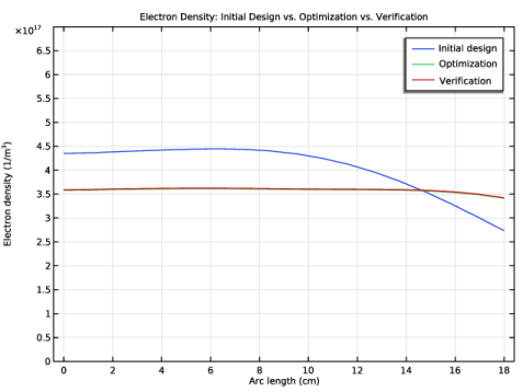
In the Settings window for 1D Plot Group, type Electron Density: Initial Design vs. Optimization vs. Verification in the Label text field.
|
|
3
|
|
1
|
Right-click Electron Density: Initial Design vs. Optimization vs. Verification and choose Line Graph.
|
|
3
|
|
4
|
Select the Show legends checkbox.
|
|
5
|
|
7
|
|
1
|
|
2
|
|
3
|
|
4
|
Locate the Legends section. In the table, enter the following settings:
|
|
1
|
|
2
|
|
3
|
|
4
|
Locate the Legends section. In the table, enter the following settings:
|
|
5
|
|
1
|
In the Model Builder window, click Electron Density: Initial Design vs. Optimization vs. Verification.
|
|
2
|
|
3
|
Select the Manual axis limits checkbox.
|
|
4
|
|
5
|
|
6
|
|
1
|
Right-click Electron Density: Initial Design vs. Optimization vs. Verification and choose Duplicate.
|
|
2
|
In the Model Builder window, click Electron Density: Initial Design vs. Optimization vs. Verification 1.
|
|
3
|
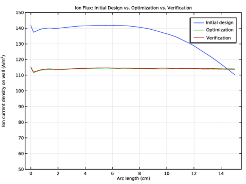
In the Settings window for 1D Plot Group, type Ion Flux: Initial Design vs. Optimization vs. Verification in the Label text field.
|
|
1
|
|
2
|
|
3
|
Click to select the
|
|
4
|
Click
|
|
6
|
|
7
|
|
8
|
|
1
|
|
2
|
|
3
|
Click to select the
|
|
4
|
Click
|
|
6
|
|
7
|
|
8
|
|
1
|
|
2
|
|
3
|
Click to select the
|
|
4
|
Click
|
|
6
|
|
7
|
|
8
|
|
1
|
|
2
|
|
3
|
|
4
|
|
5
|
|
6
|
|
1
|
|
2
|
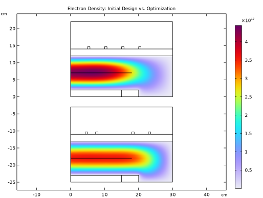
In the Settings window for 2D Plot Group, type Electron Density: Initial Design vs. Optimization in the Label text field.
|
|
3
|
|
1
|
|
2
|
|
3
|
|
1
|
In the Model Builder window, right-click Electron Density: Initial Design vs. Optimization and choose Surface.
|
|
2
|
|
3
|
|
4
|
|
1
|
|
2
|
|
3
|
|
4
|
Locate the Scale section.
|
|
5
|
|
1
|
In the Model Builder window, right-click Electron Density: Initial Design vs. Optimization and choose Line.
|
|
2
|
|
3
|
|
4
|
|
5
|
|
6
|
|
1
|
|
2
|
|
3
|
|
4
|
Locate the Scale section.
|
|
5
|
|
6
|
|
7
|
|
1
|
In the Model Builder window, right-click Electron Density: Initial Design vs. Optimization and choose Duplicate.
|
|
2
|
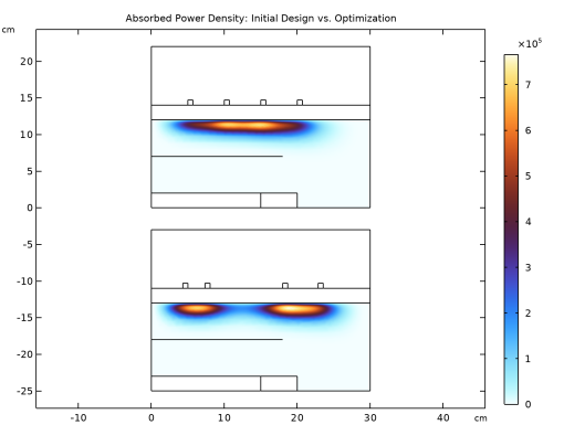
In the Settings window for 2D Plot Group, type Absorbed Power Density: Initial Design vs. Optimization in the Label text field.
|
|
1
|
In the Model Builder window, expand the Absorbed Power Density: Initial Design vs. Optimization node, then click Surface 1.
|
|
2
|
|
3
|
|
4
|
|
1
|
|
2
|
|
3
|
|
1
|
|
1
|
|
3
|