PDF

Model of a CF4/O2 Inductively Coupled Plasma Reactor
Introduction
This tutorial model studies an inductively coupled plasma (ICP) reactor in a mixture of CF4/O2. The plasma chemistry is based on Ref. 1 and the electron impact reactions are taken from LxCat (Ref. 2, Ref. 3, and Ref. 4). The plasma model is solved self-consistently with the Magnetic Fields, Laminar Flow and Heat Transfer in Fluids interfaces.
Model Definition
Electron transport is modeled by solving the continuity equation, the momentum equation under the drift-diffusion approximation, and the mean electron energy equation (for detailed information on electron transport, see Theory for the Drift Diffusion Interface in the Plasma Module User’s Guide)
The source coefficients in the above equations are determined by the plasma chemistry. The electron rate expression is defined as
where νe,j is the stoichiometric coefficient, and the reaction rate is defined as
where kjf is the forward rate constant and kjr is the reversed rate constant. Both the Electron Impact Reaction feature and Reaction feature can contribute to the electron rate expression. However, when using the Reaction feature it is important to note that the associated electron energy gain or loss is not included in the source term of the electron mean energy equation.
The rate constants can be computed from electron impact cross-section data
where γ = (2q/me)1/2 (SI unit: C1/2/kg1/2), me is the electron mass (SI unit: kg), ε is the electron energy (SI unit: V), σ is the electron impact collision cross section (SI unit: m2), and f is the electron energy distribution function.
When Townsend coefficients are used, the reaction rate is defined as
where αj/Nn is the reduced Townsend coefficient for reaction j (SI unit: m2) and Γe is the electron flux as defined above (SI unit: 1/(m2·s)). Townsend coefficients can increase the stability of the numerical scheme when the electron flux is field driven as is the case with DC discharges.
The total electron energy loss or gained is calculated by summing the collisional energy changes from all reactions defined with the Electron Impact Reaction feature as
where Δεj is the energy loss from reaction j (SI unit: V) and F is the Faraday constant (SI unit: C/mol). For excitation and ionization collisions Δεj corresponds to the energy of the excited state being excited/deexcited or ionized, for attachment Δεj is set to zero, and for elastic collisions
where me and mk are the electron and heavy species mass in kg, Te is the electron temperature in eV, and Tgas is the gas temperature in K.
For heavy species, the following equation is solved for the mass fraction of each species (for detailed information on the transport of the nonelectron species, see Theory for the Heavy Species Transport Interface in the Plasma Module User’s Guide):
The electrostatic field is computed using the following equation:
The space charge density ρ is automatically computed based on the plasma chemistry specified in the model using the formula
For detailed information about electrostatics see Theory for the Electrostatics Interface in the Plasma Module User’s Guide.
For a nonmagnetized, nonpolarized plasma, the induction currents are computed in the frequency domain using the equation
In the cold plasma approximation, the electromagnetic wave “sees” a plasma defined by the plasma conductivity, which is set in the Plasma Conductivity Coupling multiphysics node:
where ne is the electron density, q is the electron charge, me is the electron mass, νe is the collision frequency, and ω is the angular frequency. The Joule heating term responsible for heating the electrons is set in the Electron Heat Source multiphysics node.
boundary conditions
Electrons are lost to the wall due to random motion within a few mean free paths of the wall and gained due to secondary emission effects, resulting in the following boundary conditions for the electron and electron energy fluxes, respectively:
For the heavy species, ions are lost to the wall due to surface reactions and the fact that the electric field is directed toward the wall:
The walls of the reactor are grounded.
Plasma Chemistry
The plasma chemistry is based on Ref. 1. The electron impact cross sections used in this model are retrieved from different databases from LxCat: Ref. 2, Ref. 3, and Ref. 4. The data from Ref. 2 further refers to Ref. 5 and Ref. 6. The model includes 29 species: electrons, CF4, CF3, CF2, CF, CF3+, CF2+, CF+, F2, F2+, F, F+, F-, O2, O2+, O, O+, O-, O2*, O*, C, C+, CO2, CO2+, CO, CO+, COF, COF2, and FO.
Results and Discussion
The model contains two studies. In the first study, a base case is solved to provide initial conditions to a subsequent study where the oxygen mole fraction of the gas feed is parameterized. The ICP reactor is operated at 25 mTorr at the pump port with a mass flow of 50 SCCM. The input power is kept constant at 250 W.
Figure 1 shows the power density absorbed by the electrons by Joule heating caused by the coil induced currents. The power density has a typical profile found in ICP reactors with a maximum value just below the coil and being practically negligible in the reactor center because the electric fields are shielded by the dense plasma.
Figure 2, Figure 3, and Figure 4 show maximum values for the electron density, electron temperature, atomic oxygen number density, and atomic fluorine number density as a function of the molecular oxygen mole fraction in the reactor feed. These results are consistent with the experimental and model data of Ref. 1.
Figure 1: Power absorbed by the electrons for an oxygen mole fraction of 0.9.
Figure 2: Maximum values of electron density and electron temperature as a function of oxygen mole fraction.
Figure 3: Maximum value of atomic oxygen number density as a function of oxygen mole fraction.
Figure 4: Maximum value of atomic fluorine number density as a function of oxygen mole fraction.
References
1. T. Kimura and M. Noto, “Experimental study and global model of inductively coupled CF4/O2 discharges,” J. Appl. Phys., vol. 100, no. 063303, pp. 1–9, 2006; doi.org/10.1063/1.2345461.
2. Bordage database, www.lxcat.net, retrieved on 2025.
3. Morgan database, www.lxcat.net, retrieved on 2025.
4. Phelps database, www.lxcat.net, retrieved 2025.
5. M.C. Bordage, P. Segur, and A. Chouki, “Determination of a set of electron impact cross sections in tetrafluoromethane consistent with experimental determination of swarm parameters,” J. Appl. Phys., vol. 80, no. 3, pp. 1325–1336, 1996; doi.org/10.1063/1.362931.
6. M.C. Bordage, P. Segur, L.G. Christophorou, and J.K. Olthoff, “Boltzmann analysis of electron swarm parameters in CF4 using independently assessed electron-collision cross sections,” J. Appl. Phys., vol. 86, no. 7, pp. 3558–3566, 1999; doi.org/10.1063/1.371258.
Application Library path: Plasma_Module/Inductively_Coupled_Plasmas/icp_cf4_o2
Modeling Instructions
From the File menu, choose New.
New
In the New window, click  Model Wizard.
Model Wizard
1
In the Model Wizard window, click  2D Axisymmetric.
2
In the Select Physics tree, select Plasma > Nonisothermal Plasma Flow > Inductively Coupled Plasma.
3
Click Add.
4
Click  Study.
5
In the Select Study tree, select Preset Studies for Selected Multiphysics > Frequency–Stationary.
6
Global Definitions
Parameters 1
Import parameters to use in the model.
1
In the Model Builder window, under Global Definitions click Parameters 1.
2
In the Settings window for Parameters, locate the Parameters section.
3
Click  Load from File.
4
In the following, create a geometry for an ICP reactor.
Geometry 1
1
In the Model Builder window, under Component 1 (comp1) click Geometry 1.
2
In the Settings window for Geometry, locate the Units section.
3
From the Length unit list, choose cm.
Rectangle 1 (r1)
1
In the Geometry toolbar, click  Rectangle.
2
In the Settings window for Rectangle, locate the Size and Shape section.
3
In the Width text field, type Wc.
4
In the Height text field, type Hc.
Rectangle 2 (r2)
1
In the Geometry toolbar, click  Rectangle.
2
In the Settings window for Rectangle, locate the Size and Shape section.
3
In the Width text field, type Wc.
4
In the Height text field, type Window_thickness.
5
Locate the Position section. In the z text field, type Hc.
Rectangle 3 (r3)
1
In the Geometry toolbar, click  Rectangle.
2
In the Settings window for Rectangle, locate the Size and Shape section.
3
In the Width text field, type Wc.
4
In the Height text field, type Coil_chamber_height.
5
Locate the Position section. In the z text field, type Hc+Window_thickness.
Rectangle 4 (r4)
1
In the Geometry toolbar, click  Rectangle.
2
In the Settings window for Rectangle, locate the Size and Shape section.
3
In the Width text field, type Coil_width.
4
In the Height text field, type Coil_height.
5
Locate the Position section. In the r text field, type First_coil_r.
6
In the z text field, type Hc+Window_thickness+First_coil_z.
7
Click  Build All Objects.
Array 1 (arr1)
1
In the Geometry toolbar, click  Transforms and choose Array.
2
In the Settings window for Array, locate the Size section.
3
In the r size text field, type 4.
4
Locate the Displacement section. In the r text field, type Coils_spacing.
5
6
Click  Build All Objects.
Rectangle 5 (r5)
1
In the Geometry toolbar, click  Rectangle.
2
In the Settings window for Rectangle, locate the Size and Shape section.
3
In the Width text field, type Ww.
4
In the Height text field, type Wh.
Rectangle 6 (r6)
1
In the Geometry toolbar, click  Rectangle.
2
In the Settings window for Rectangle, locate the Size and Shape section.
3
In the Width text field, type Inw.
4
In the Height text field, type Inh.
5
Locate the Position section. In the r text field, type Wc-Inw.
6
In the z text field, type Hc-Inh.
Line Segment 1 (ls1)
1
In the Geometry toolbar, click  More Primitives and choose Line Segment.
2
On the object r5, select Point 4 only.
3
In the Settings window for Line Segment, locate the Endpoint section.
4
From the Specify list, choose Coordinates.
5
In the r text field, type 15.
6
In the z text field, type Wh.
Line Segment 2 (ls2)
1
In the Geometry toolbar, click  More Primitives and choose Line Segment.
2
In the Settings window for Line Segment, locate the Starting Point section.
3
From the Specify list, choose Coordinates.
4
In the r text field, type Wc-Inw.
5
In the z text field, type Hc-Inh+1.5[cm].
6
Locate the Endpoint section. From the Specify list, choose Coordinates.
7
In the r text field, type Wc-Inw.
8
In the z text field, type Hc-Inh+3.5[cm].
9
Click  Build All Objects.
Geometry 1
In the Model Builder window, collapse the Component 1 (comp1) > Geometry 1 node.
Set material properties to be used by the different physics interfaces in this model.
Add Material
1
In the Materials toolbar, click  Add Material to open the Add Material window.
2
Go to the Add Material window.
3
In the tree, select Built-in > Air.
4
Click the Add to Component button in the window toolbar.
5
In the tree, select Built-in > Glass (quartz).
6
Click the Add to Component button in the window toolbar.
7
In the tree, select Built-in > Copper.
8
Click the Add to Component button in the window toolbar.
9
In the Materials toolbar, click  Add Material to close the Add Material window.
Materials
Copper (mat3)
1
Click the  Zoom Extents button in the Graphics toolbar.
2
Glass (quartz) (mat2)
1
In the Model Builder window, click Glass (quartz) (mat2).
2
Air (mat1)
1
In the Model Builder window, click Air (mat1).
2
In the Settings window for Material, locate the Geometric Entity Selection section.
3
Click  Clear Selection.
4
Define explicit selections to be used later for boundary conditions and meshing.
Definitions
Coil
1
In the Definitions toolbar, click  Explicit.
2
In the Settings window for Explicit, type Coil in the Label text field.
3
Coil Boundaries
1
Right-click Coil and choose Duplicate.
2
In the Settings window for Explicit, type Coil Boundaries in the Label text field.
3
Locate the Output Entities section. From the Output entities list, choose Adjacent boundaries.
Walls
1
In the Definitions toolbar, click  Explicit.
2
In the Settings window for Explicit, type Walls in the Label text field.
3
Locate the Input Entities section. From the Geometric entity level list, choose Boundary.
4
Define a Maximum operator to be used during plotting.
Maximum 1 (maxop1)
1
In the Definitions toolbar, click  Nonlocal Couplings and choose Maximum.
2
In the Magnetic Fields interface the first thing to do is to set the domains where the physics is to be solved. After, add a Coil feature, select the coil domain, and set the coil power.
Magnetic Fields (mf)
1
In the Model Builder window, under Component 1 (comp1) click Magnetic Fields (mf).
2
In the Settings window for Magnetic Fields, locate the Domain Selection section.
3
Click  Clear Selection.
4
Domain Coil 1
1
In the Physics toolbar, click  Domains and choose Domain Coil.
2
In the Settings window for Domain Coil, locate the Domain Selection section.
3
From the Selection list, choose Coil.
4
Locate the Coil section. Select the Coil group checkbox.
5
From the Coil excitation list, choose Power.
6
In the Pcoil text field, type Pw.
Magnetic Fields (mf)
In the Model Builder window, collapse the Component 1 (comp1) > Magnetic Fields (mf) node.
Set the domains where the Heat Transfer in Fluids interface is to be solved and set a constant temperature as boundary condition.
Heat Transfer in Fluids (ht)
1
In the Model Builder window, under Component 1 (comp1) click Heat Transfer in Fluids (ht).
2
In the Settings window for Heat Transfer in Fluids, locate the Domain Selection section.
3
Click  Clear Selection.
4
Temperature 1
1
In the Physics toolbar, click  Boundaries and choose Temperature.
2
In the Settings window for Temperature, locate the Boundary Selection section.
3
From the Selection list, choose Walls.
In the Laminar Flow interface, set the domain where the physics is to be solved, and add an inlet and outlet to the system.
Laminar Flow (spf)
1
In the Model Builder window, under Component 1 (comp1) click Laminar Flow (spf).
2
In the Settings window for Laminar Flow, locate the Domain Selection section.
3
Click  Clear Selection.
4
5
Locate the Physical Model section. In the pref text field, type p0.
Inlet 1
1
In the Physics toolbar, click  Boundaries and choose Inlet.
2
3
In the Settings window for Inlet, locate the Boundary Condition section.
4
5
Locate the Mass Flow section. From the Mass flow type list, choose Standard flow rate (SCCM).
6
In the Qsccm text field, type Qf.
Outlet 1
1
In the Physics toolbar, click  Boundaries and choose Outlet.
2
Laminar Flow (spf)
In the Model Builder window, collapse the Component 1 (comp1) > Laminar Flow (spf) node.
Heat Transfer in Fluids (ht)
In the Model Builder window, collapse the Component 1 (comp1) > Heat Transfer in Fluids (ht) node.
Plasma (plas)
Add isotropic diffusion for ions because the density of the negative ions can drop sharply when approaching the reactor edges and cause instability.
1
Click the  Show More Options button in the Model Builder toolbar.
2
In the Show More Options dialog, select Physics > Stabilization in the tree.
3
4
5
In the Model Builder window, under Component 1 (comp1) click Plasma (plas).
6
In the Settings window for Plasma, locate the Domain Selection section.
7
Click  Clear Selection.
8
9
Locate the Transport Settings section. Select the Mixture diffusion correction checkbox.
10
Click to expand the Inconsistent Stabilization section. Select the Isotropic diffusion for ions checkbox.
11
In the δid,i text field, type 0.1.
Plasma Model 1
1
In the Model Builder window, under Component 1 (comp1) > Plasma (plas) click Plasma Model 1.
2
In the Settings window for Plasma Model, locate the Electron Density and Energy section.
3
From the Electron transport properties list, choose From electron impact reactions to estimate the electron transport parameters from the existent reactions.
Initial Values 1
1
In the Model Builder window, click Initial Values 1.
2
In the Settings window for Initial Values, locate the Initial Values section.
3
In the ne,0 text field, type 1E15[1/m^3].
4
In the ε0 text field, type 2[V].
The Plasma Chemistry Import Feature
The next steps have instructions to use the Plasma Chemistry Import feature to import a file that automatically creates the CF4/O2 plasma chemistry.
The following is set or created automatically:
a
b
c
d
The documentation accompanying the Plasma Chemistry Import feature contains more information about the file structure and what can be set automatically.
Plasma Chemistry Import 1
1
In the Physics toolbar, click  Global and choose Plasma Chemistry Import.
2
In the Settings window for Plasma Chemistry Import, locate the Plasma Chemistry Import section.
3
Click  Browse.
4
5
Click  Import.
Select where the surface reactions are to be used.
Surface Reactions - Ions
1
In the Model Builder window, click Surface Reactions - Ions.
2
In the Settings window for Surface Reaction Group, locate the Boundary Selection section.
3
From the Selection list, choose Walls.
Surface Reactions - Neutrals
1
In the Model Builder window, click Surface Reactions - Neutrals.
2
In the Settings window for Surface Reaction Group, locate the Boundary Selection section.
3
From the Selection list, choose Walls.
4
Add boundary conditions for the electron transport equations, Poisson’s equation.
Wall 1
1
In the Physics toolbar, click  Boundaries and choose Wall.
2
In the Settings window for Wall, locate the Boundary Selection section.
3
From the Selection list, choose Walls.
Ground 1
1
In the Physics toolbar, click  Boundaries and choose Ground.
2
In the Settings window for Ground, locate the Boundary Selection section.
3
From the Selection list, choose Walls.
Add an Inlet feature to set the mole fraction of CF4 and O2 in the feed gas. The mole fraction of all other neutral species (fragments, excited states and others) should be fixed to a small number to say that they have negligible presence in the feed gas.
Inflow 1
1
In the Physics toolbar, click  Boundaries and choose Inflow.
2
In the Settings window for Inflow, locate the Inflow section.
3
4
5
6
7
8
9
10
11
12
13
14
15
16
17
18
19
20
21
22
23
24
25
26
27
28
29
30
31
32
33
34
35
Use the Outflow feature to specify that the neutral species have no transport due to diffusion at the outlet.
Outflow 1
1
In the Physics toolbar, click  Boundaries and choose Outflow.
2
In the following, set the CF4 mass fraction to be computed from a mass constraint, set species initial conditions, and set additional entropy to some excited states.
Species: CF4
1
In the Model Builder window, expand the Component 1 (comp1) > Plasma (plas) > Group - Species node, then click Species: CF4.
2
In the Settings window for Species, locate the Species Formula section.
3
Select the From mass constraint checkbox.
Species: F-
1
In the Model Builder window, click Species: F-.
2
In the Settings window for Species, locate the General Parameters section.
3
In the n0 text field, type 1E10[1/m^3].
Species: CF3+
1
In the Model Builder window, click Species: CF3+.
2
In the Settings window for Species, locate the Species Formula section.
3
Select the Initial value from electroneutrality constraint checkbox.
Species: CF2+
1
In the Model Builder window, click Species: CF2+.
2
In the Settings window for Species, locate the General Parameters section.
3
In the n0 text field, type 1E10[1/m^3].
Species: CF+
1
In the Model Builder window, click Species: CF+.
2
In the Settings window for Species, locate the General Parameters section.
3
In the n0 text field, type 1E10[1/m^3].
Species: O+
1
In the Model Builder window, click Species: O+.
2
In the Settings window for Species, locate the General Parameters section.
3
In the n0 text field, type 1E10[1/m^3].
4
Click to expand the Species Thermodynamic Parameters section. In the Δh text field, type 13.618.
Species: O2
1
In the Model Builder window, click Species: O2.
2
In the Settings window for Species, locate the General Parameters section.
3
In the x0 text field, type xO2.
Species: O-
1
In the Model Builder window, click Species: O-.
2
In the Settings window for Species, locate the General Parameters section.
3
In the n0 text field, type 1E10[1/m^3].
Species: O2+
1
In the Model Builder window, click Species: O2+.
2
In the Settings window for Species, locate the General Parameters section.
3
In the n0 text field, type 1E10[1/m^3].
4
Locate the Species Thermodynamic Parameters section. In the Δh text field, type 12.06.
Species: F2+
1
In the Model Builder window, click Species: F2+.
2
In the Settings window for Species, locate the General Parameters section.
3
In the n0 text field, type 1E10[1/m^3].
4
Locate the Species Thermodynamic Parameters section. In the Δh text field, type 15.69.
Species: F+
1
In the Model Builder window, click Species: F+.
2
In the Settings window for Species, locate the Species Thermodynamic Parameters section.
3
In the Δh text field, type 17.687.
4
Locate the General Parameters section. In the n0 text field, type 1E10[1/m^3].
Species: CO2+
1
In the Model Builder window, click Species: CO2+.
2
In the Settings window for Species, locate the General Parameters section.
3
In the n0 text field, type 1E10[1/m^3].
4
Locate the Species Thermodynamic Parameters section. In the Δh text field, type 13.3.
Species: CO+
1
In the Model Builder window, click Species: CO+.
2
In the Settings window for Species, locate the Species Thermodynamic Parameters section.
3
In the Δh text field, type 14.
4
Locate the General Parameters section. In the n0 text field, type 1E10[1/m^3].
Species: C+
1
In the Model Builder window, click Species: C+.
2
In the Settings window for Species, locate the General Parameters section.
3
In the n0 text field, type 1E10[1/m^3].
4
Locate the Species Thermodynamic Parameters section. In the Δh text field, type 11.26.
Plasma (plas)
Group - Species
1
In the Model Builder window, collapse the Component 1 (comp1) > Plasma (plas) > Group - Species node.
2
In the Model Builder window, collapse the Plasma (plas) node.
Mesh 1
1
In the Model Builder window, under Component 1 (comp1) click Mesh 1.
2
In the Settings window for Mesh, locate the Physics-Controlled Mesh section.
3
In the table, clear the Use checkbox for Plasma (plas).
4
Locate the Sequence Type section. From the list, choose User-controlled mesh.
Size 1
1
In the Model Builder window, under Component 1 (comp1) > Mesh 1 click Size 1.
2
In the Settings window for Size, locate the Element Size section.
3
From the Predefined list, choose Finer.
Free Triangular 1
1
In the Model Builder window, click Free Triangular 1.
2
In the Settings window for Free Triangular, locate the Domain Selection section.
3
Click  Clear Selection.
4
Boundary Layer Properties 1
1
In the Model Builder window, expand the Component 1 (comp1) > Mesh 1 > Boundary Layers 1 node, then click Boundary Layer Properties 1.
2
In the Settings window for Boundary Layer Properties, locate the Layers section.
3
In the Number of layers text field, type 4.
4
In the Stretching factor text field, type 1.4.
5
In the Thickness adjustment factor text field, type 1.
Mapped 1
1
In the Mesh toolbar, click  Mapped.
2
In the Settings window for Mapped, locate the Domain Selection section.
3
From the Geometric entity level list, choose Domain.
4
From the Selection list, choose Coil.
Distribution 1
1
Right-click Mapped 1 and choose Distribution.
2
In the Settings window for Distribution, locate the Distribution section.
3
From the Distribution type list, choose Predefined.
4
In the Number of elements text field, type 30.
5
In the Element ratio text field, type 20.
6
From the Growth rate list, choose Exponential.
7
Select the Symmetric distribution checkbox.
8
Locate the Boundary Selection section. From the Selection list, choose Coil Boundaries.
Mapped 1
1
In the Model Builder window, right-click Mapped 1 and choose Move Up.
2
Right-click Mapped 1 and choose Move Up.
3
In the Settings window for Mapped, click  Build All.
A first study is used to provide initial conditions to subsequent studies.
Base Case
1
In the Model Builder window, click Study 1.
2
In the Settings window for Study, type Base Case in the Label text field.
3
In the Study toolbar, click  Get Initial Value.
Results
Electric Potential (plas), Electron Density (plas), Electron Temperature (plas), Magnetic Flux Density (mf), Magnetic Flux Density, Revolved Geometry (mf), Pressure (spf), Temperature (ht), Velocity (spf), Velocity, 3D (spf)
Right-click and choose Group.
Base Case
In the Settings window for Group, type Base Case in the Label text field.
Base Case
Step 1: Frequency–Stationary
1
In the Model Builder window, expand the Base Case > Solver Configurations node, then click Base Case > Step 1: Frequency–Stationary.
2
In the Settings window for Frequency–Stationary, locate the Study Settings section.
3
In the Frequency text field, type 13.56e6.
Solution 1 (sol1)
1
In the Model Builder window, expand the Base Case > Solver Configurations > Solution 1 (sol1) > Stationary Solver 1 node, then click Fully Coupled 1.
2
In the Settings window for Fully Coupled, click to expand the Results While Solving section.
3
Select the Plot checkbox.
4
Results
Electron Density (plas)
Add a second study to do a parameterization on the oxygen mole fraction. Since we already have a previous solution the initial damping factor can be set to 1.
Add Study
1
In the Home toolbar, click  Add Study to open the Add Study window.
2
Go to the Add Study window.
3
Find the Studies subsection. In the Select Study tree, select Preset Studies for Selected Multiphysics > Frequency–Stationary.
4
Click the Add Study button in the window toolbar.
5
In the Home toolbar, click  Add Study to close the Add Study window.
Study 2
Step 1: Frequency–Stationary
1
In the Settings window for Frequency–Stationary, locate the Study Settings section.
2
In the Frequency text field, type 13.56e6.
3
Click to expand the Values of Dependent Variables section. Find the Initial values of variables solved for subsection. From the Settings list, choose User controlled.
4
From the Method list, choose Solution.
5
From the Study list, choose Base Case, Frequency–Stationary.
6
In the Model Builder window, click Study 2.
7
In the Settings window for Study, type xO2 Sweep in the Label text field.
8
In the Study toolbar, click  Get Initial Value.
Results
Electric Potential (plas) 1, Electron Density (plas) 1, Electron Temperature (plas) 1, Magnetic Flux Density (mf) 1, Magnetic Flux Density, Revolved Geometry (mf) 1, Pressure (spf) 1, Temperature (ht) 1, Velocity (spf) 1, Velocity, 3D (spf) 1
Right-click and choose Group.
xO2 Sweep
In the Settings window for Group, type xO2 Sweep in the Label text field.
xO2 Sweep
Solver Configurations
In the Model Builder window, expand the xO2 Sweep > Solver Configurations node.
Solution 2 (sol2)
1
In the Model Builder window, expand the xO2 Sweep > Solver Configurations > Solution 2 (sol2) > Stationary Solver 1 node, then click Fully Coupled 1.
2
In the Settings window for Fully Coupled, click to expand the Method and Termination section.
3
In the Initial damping factor text field, type 1.
4
Locate the Results While Solving section. Select the Plot checkbox.
5
Parametric Sweep
1
In the Study toolbar, click  Parametric Sweep.
2
In the Settings window for Parametric Sweep, locate the Study Settings section.
3
4
5
Click to expand the Advanced Settings section. Select the Reuse solution from previous step checkbox.
6
In the Study toolbar, click  Compute.
Prepare plots to show the electron density, electron temperature, F number density, and O number density as functions of the O2 mole fraction.
Results
Electron Density and Temperature vs. xO2
1
In the Results toolbar, click  1D Plot Group.
2
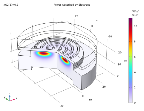
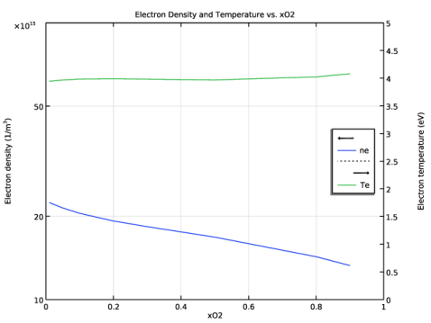
In the Settings window for 1D Plot Group, type Electron Density and Temperature vs. xO2 in the Label text field.
3
Locate the Data section. From the Dataset list, choose xO2 Sweep/Solution 2 (sol2).
Global 1
1
Right-click Electron Density and Temperature vs. xO2 and choose Global.
2
In the Settings window for Global, locate the y-Axis Data section.
3
4
Click to expand the Legends section. From the Legends list, choose Manual.
5
Global 2
1
Right-click Global 1 and choose Duplicate.
2
In the Settings window for Global, locate the y-Axis Data section.
3
4
Locate the Legends section. In the table, enter the following settings:
Electron Density and Temperature vs. xO2
1
In the Model Builder window, click Electron Density and Temperature vs. xO2.
2
In the Settings window for 1D Plot Group, click to expand the Title section.
3
From the Title type list, choose Label.
4
Locate the Plot Settings section. Select the Two y-axes checkbox.
5
In the table, select the Plot on secondary y-axis checkbox for Global 2.
6
Select the y-axis label checkbox. In the associated text field, type Electron density (1/m<sup>3</sup>).
7
Select the Secondary y-axis label checkbox. In the associated text field, type Electron temperature (eV).
8
Locate the Axis section. Select the y-axis log scale checkbox.
9
Select the Manual axis limits checkbox.
10
In the x minimum text field, type 0.
11
In the x maximum text field, type 1.
12
In the y minimum text field, type 1e16.
13
In the y maximum text field, type 1e17.
14
In the Secondary y minimum text field, type 0.
15
In the Secondary y maximum text field, type 5.
16
Locate the Legend section. From the Position list, choose Middle right.
17
In the Electron Density and Temperature vs. xO2 toolbar, click  Plot.
O Density vs. xO2
1
In the Results toolbar, click  1D Plot Group.
2
In the Settings window for 1D Plot Group, type O Density vs. xO2 in the Label text field.
3
Locate the Data section. From the Dataset list, choose xO2 Sweep/Solution 2 (sol2).
Global 1
1
Right-click O Density vs. xO2 and choose Global.
2
In the Settings window for Global, locate the y-Axis Data section.
3
O Density vs. xO2
1
In the Model Builder window, click O Density vs. xO2.
2
In the Settings window for 1D Plot Group, locate the Title section.
3
From the Title type list, choose None.
4
Locate the Plot Settings section.
5
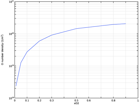
Select the y-axis label checkbox. In the associated text field, type O number density (1/m<sup>3</sup>).
6
Locate the Axis section. Select the y-axis log scale checkbox.
7
Select the Manual axis limits checkbox.
8
In the x minimum text field, type 0.
9
In the x maximum text field, type 1.
10
In the y minimum text field, type 1e18.
11
In the y maximum text field, type 1e21.
12
Locate the Legend section. Clear the Show legends checkbox.
13
In the O Density vs. xO2 toolbar, click  Plot.
F Density vs. xO2
1
Right-click O Density vs. xO2 and choose Duplicate.
2
In the Settings window for 1D Plot Group, type F Density vs. xO2 in the Label text field.
3
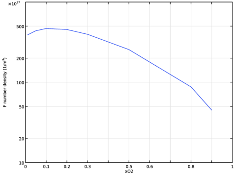
Locate the Plot Settings section. In the y-axis label text field, type F number density (1/m<sup>3</sup>).
4
Locate the Axis section. In the y maximum text field, type 1e20.
Global 1
1
In the Model Builder window, expand the F Density vs. xO2 node, then click Global 1.
2
In the Settings window for Global, locate the y-Axis Data section.
3
4
In the F Density vs. xO2 toolbar, click  Plot.
Prepare a plot to show the power absorbed by electrons. First, create a dataset with a selection of the plasma domain only.
Revolution 2D 4
1
In the Model Builder window, expand the Results > Datasets node.
2
Right-click Results > Datasets > Revolution 2D 3 and choose Duplicate.
Selection
1
In the Results toolbar, click  Attributes and choose Selection.
2
In the Settings window for Selection, locate the Geometric Entity Selection section.
3
From the Geometric entity level list, choose Domain.
4
Power Absorbed by Electrons
1
In the Results toolbar, click  3D Plot Group.
2
In the Settings window for 3D Plot Group, type Power Absorbed by Electrons in the Label text field.
3
Locate the Data section. From the Dataset list, choose Revolution 2D 1.
Volume 1
1
Right-click Power Absorbed by Electrons and choose Volume.
2
In the Settings window for Volume, locate the Data section.
3
From the Dataset list, choose Revolution 2D 4.
4
Locate the Expression section. In the Expression text field, type mf.Qrh.
Power Absorbed by Electrons
1
In the Model Builder window, click Power Absorbed by Electrons.
2
In the Settings window for 3D Plot Group, click to expand the Title section.
3
From the Title type list, choose Label.
4
Locate the Color Legend section. Select the Show units checkbox.
5
In the Power Absorbed by Electrons toolbar, click  Plot.