
|
|
|


|
|
|||
|
|
|||
|
e+O2=>e+O+O
|
|||
|
e+O=>e+O(1D)
|
|||
|
e+O-=>O+e+e
|
|
Ar+=>Ar
|
||||
|
O-=>O
|
||||
|
O+=>O
|
|
•
|
Increase the negative ion temperature of about 0.3 eV. An higher ion temperature makes the transport numerical easier. The ion temperature is defined in the section Mobility and Diffusivity Expressions in the species Settings. By default the ion temperature is the gas temperature.
|
|
•
|
Enable Isotropic diffusion for ions in the Inconsistent Stabilization section (the stabilization sections are visible when Stabilization is selected in Show More Options). This option adds artificial diffusion to all ions and helps smoothing the sharp transition of the negative ion density between the electropositive edge and the electronegative core, and also increase the density of the negative ions in the electropositive edge effectively increasing its losses by transport. This option should be used very carefully since completely wrong results can be obtained if too much diffusion is used (the tuning parameter for ions should not be larger than 0.1). A useful strategy is to start with a large Tuning parameter for ions (for example, 0.5) and ramp it down using an Auxiliary sweep.
|
|
1
|
|
2
|
|
3
|
Click Add.
|
|
4
|
Click
|
|
5
|
|
6
|
Click
|
|
1
|
|
2
|
|
3
|
|
1
|
|
2
|
|
3
|
|
4
|
|
1
|
|
2
|
|
3
|
|
4
|
|
5
|
|
1
|
|
2
|
|
3
|
|
4
|
|
1
|
|
2
|
Select the object r3 only.
|
|
3
|
|
4
|
|
5
|
|
1
|
|
2
|
|
3
|
|
4
|
|
1
|
|
2
|
|
3
|
|
4
|
|
5
|
|
1
|
|
2
|
|
3
|
|
4
|
|
5
|
|
6
|
|
1
|
|
2
|
|
3
|
|
4
|
|
5
|
|
6
|
|
7
|
|
8
|
|
9
|
Click
|
|
1
|
|
2
|
|
1
|
|
2
|
|
4
|
|
1
|
|
2
|
|
1
|
|
2
|
|
3
|
|
1
|
|
1
|
|
2
|
Go to the Add Material window.
|
|
3
|
|
4
|
Click the Add to Component button in the window toolbar.
|
|
5
|
|
6
|
Click the Add to Component button in the window toolbar.
|
|
7
|
|
8
|
Click the Add to Component button in the window toolbar.
|
|
9
|
|
1
|
|
2
|
Click
|
|
1
|
|
1
|
|
2
|
|
3
|
|
a
|
Species properties using Preset species data
|
|
1
|
|
2
|
|
3
|
Click
|
|
4
|
Browse to the model’s Application Libraries folder and double-click the file Ar_O2_plasma_chemistry.txt.
|
|
5
|
Click
|
|
6
|
|
7
|
|
8
|
Click
|
|
10
|
|
11
|
|
12
|
|
13
|
Click OK.
|
|
14
|
|
15
|
Select the Isotropic diffusion for ions checkbox.
|
|
16
|
|
17
|
|
1
|
|
2
|
|
3
|
|
1
|
|
2
|
|
3
|
|
1
|
In the Model Builder window, expand the Component 1 (comp1) > Plasma (plas) > Group - Species node, then click Species: O2.
|
|
2
|
|
3
|
|
1
|
|
2
|
|
3
|
|
1
|
|
2
|
|
3
|
|
1
|
|
2
|
|
3
|
Select the Initial value from electroneutrality constraint checkbox.
|
|
1
|
|
2
|
|
3
|
|
1
|
|
2
|
|
3
|
Select the From mass constraint checkbox.
|
|
1
|
|
3
|
|
4
|
Click
|
|
1
|
|
1
|
In the Model Builder window, under Component 1 (comp1) > Plasma (plas) > Group - Species click Species: Ar+.
|
|
2
|
|
3
|
|
1
|
|
2
|
|
3
|
|
1
|
|
2
|
|
3
|
|
1
|
|
2
|
|
3
|
|
1
|
|
2
|
|
3
|
|
1
|
|
2
|
|
3
|
|
1
|
|
2
|
|
3
|
|
1
|
|
2
|
|
3
|
|
1
|
|
2
|
|
3
|
|
4
|
|
1
|
|
2
|
|
3
|
|
1
|
|
2
|
|
3
|
|
1
|
|
1
|
|
2
|
|
3
|
|
4
|
|
5
|
|
6
|
|
1
|
|
2
|
|
3
|
Click
|
|
1
|
|
2
|
|
3
|
|
4
|
|
1
|
|
2
|
|
3
|
Click
|
|
5
|
|
1
|
|
3
|
|
4
|
From the list, choose Mass flow.
|
|
5
|
|
6
|
|
1
|
|
1
|
|
2
|
|
3
|
|
5
|
|
1
|
|
2
|
|
3
|
|
1
|
|
2
|
|
3
|
|
4
|
|
6
|
|
7
|
|
1
|
|
2
|
|
3
|
|
4
|
|
1
|
|
2
|
|
3
|
|
4
|
|
5
|
|
6
|
|
7
|
Select the Symmetric distribution checkbox.
|
|
1
|
|
2
|
|
3
|
|
4
|
|
5
|
|
1
|
|
2
|
|
3
|
|
5
|
Click
|
|
1
|
|
2
|
|
3
|
|
1
|
In the Model Builder window, expand the Base Case > Solver Configurations node, then click Base Case > Step 1: Frequency–Stationary.
|
|
2
|
|
3
|
|
1
|
In the Model Builder window, expand the Base Case > Solver Configurations > Solution 1 (sol1) > Stationary Solver 1 node, then click Fully Coupled 1.
|
|
2
|
|
3
|
Select the Plot checkbox.
|
|
4
|
Click
|
|
1
|
|
2
|
Go to the Add Study window.
|
|
3
|
Find the Studies subsection. In the Select Study tree, select Preset Studies for Selected Multiphysics > Frequency–Stationary.
|
|
4
|
Click the Add Study button in the window toolbar.
|
|
5
|
|
1
|
|
2
|
|
3
|
Click to expand the Values of Dependent Variables section. Find the Initial values of variables solved for subsection. From the Settings list, choose User controlled.
|
|
4
|
|
5
|
|
6
|
|
7
|
Click
|
|
9
|
Click
|
|
10
|
|
11
|
|
12
|
|
13
|
Click Replace.
|
|
14
|
|
15
|
|
16
|
|
1
|
In the Model Builder window, expand the Power Sweep > Solver Configurations node, then click Results > Group 2.
|
|
2
|
|
1
|
In the Model Builder window, expand the Power Sweep > Solver Configurations > Solution 2 (sol2) > Stationary Solver 1 node, then click Fully Coupled 1.
|
|
2
|
|
3
|
|
4
|
|
6
|
|
1
|
|
2
|
Go to the Add Study window.
|
|
3
|
Find the Studies subsection. In the Select Study tree, select Preset Studies for Selected Multiphysics > Frequency–Stationary.
|
|
4
|
Click the Add Study button in the window toolbar.
|
|
5
|
|
1
|
|
2
|
|
3
|
Locate the Values of Dependent Variables section. Find the Initial values of variables solved for subsection. From the Settings list, choose User controlled.
|
|
4
|
|
5
|
|
6
|
|
7
|
|
8
|
|
9
|
Click
|
|
12
|
Click
|
|
13
|
|
14
|
|
15
|
|
16
|
Click Replace.
|
|
17
|
|
18
|
Click
|
|
20
|
|
21
|
|
22
|
|
1
|
In the Model Builder window, expand the xO2 Sweep > Solver Configurations node, then click Results > Group 3.
|
|
2
|
|
1
|
In the Model Builder window, expand the xO2 Sweep > Solver Configurations > Solution 3 (sol3) > Stationary Solver 1 node, then click Fully Coupled 1.
|
|
2
|
|
3
|
|
4
|
|
6
|
|
1
|
|
2
|
|
3
|
|
4
|
|
1
|
|
2
|
|
3
|
|
4
|
|
1
|
|
2
|
|
3
|
|
4
|
|
1
|
|
2
|
|
3
|
|
4
|
|
1
|
|
3
|
|
1
|
|
2
|
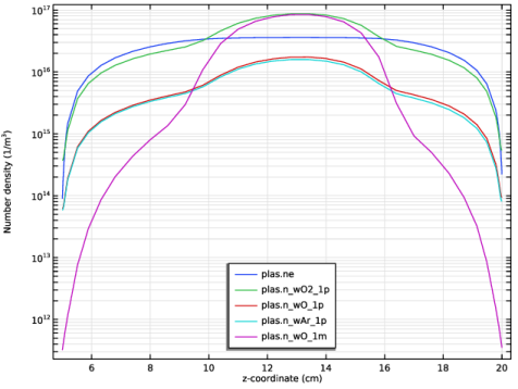
In the Settings window for 1D Plot Group, type Charged Species Along Axis-of-Symmetry in the Label text field.
|
|
3
|
|
4
|
|
5
|
|
6
|
Locate the Plot Settings section.
|
|
7
|
Select the y-axis label checkbox. In the associated text field, type Number density (1/m<sup>3</sup>).
|
|
8
|
|
1
|
|
3
|
|
4
|
|
5
|
|
6
|
|
7
|
|
8
|
Select the Expression checkbox.
|
|
1
|
|
2
|
|
3
|
|
1
|
|
2
|
|
3
|
|
1
|
|
2
|
|
3
|
|
1
|
|
2
|
|
3
|
|
4
|
|
1
|
|
2
|
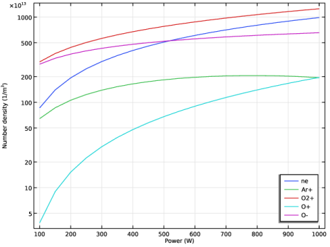
In the Settings window for 1D Plot Group, type Space Averaged Charged Species vs. Power in the Label text field.
|
|
3
|
|
4
|
|
5
|
Locate the Plot Settings section.
|
|
6
|
|
7
|
Select the y-axis label checkbox. In the associated text field, type Number density (1/m<sup>3</sup>).
|
|
8
|
|
1
|
|
2
|
|
4
|
|
5
|
|
6
|
|
1
|
|
2
|
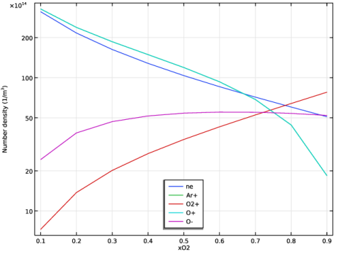
In the Settings window for 1D Plot Group, type Space Averaged Charged Species vs. xO2 in the Label text field.
|
|
3
|
|
4
|
|
5
|
|
6
|
Locate the Plot Settings section.
|
|
7
|
|
8
|
Select the y-axis label checkbox. In the associated text field, type Number density (1/m<sup>3</sup>).
|
|
9
|
|
1
|
|
2
|
|
4
|
|
5
|
|
6
|
|
7
|