|
|
|




 .
. .
.





 ,
,







 ,
, .
.
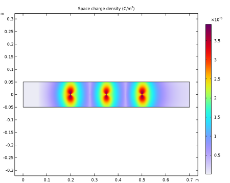
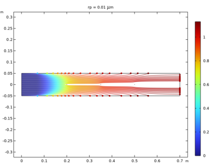
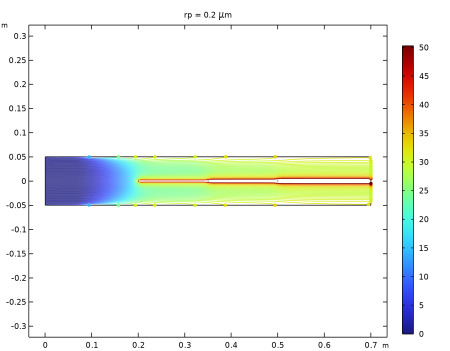
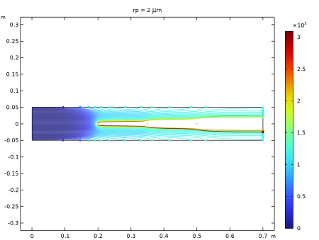
|
•
|
A Stationary study that couples the Laminar Flow (spf), Electrostatics (es) and Charge Transport (ct) interfaces.
|
|
•
|
A Time Dependent study that solves for the particle trajectories using the Particle Tracing for Fluid Flow (fpt) interface to obtain the particle collection efficiency.
|
|
1
|
In the Model Wizard window, Select the Laminar Flow (spf) interface and Corona Discharge to compute the fluid velocity, the electric field, and the space charge density that are necessary for the Particle Tracing for Fluid Flow (fpt) interface to compute the particle charging and trajectories.
|
|
2
|
click
 2D. 2D. |
|
3
|
|
4
|
Click Add.
|
|
5
|
|
6
|
Click Add.
|
|
7
|
Click
 Study. Study. |
|
8
|
|
9
|
Click
 Done. Done. |
|
1
|
|
2
|
|
1
|
|
2
|
|
3
|
|
4
|
|
5
|
|
1
|
|
2
|
|
3
|
|
4
|
|
1
|
|
2
|
Select the object c1 only.
|
|
3
|
|
4
|
|
5
|
|
1
|
|
2
|
Select the object r1 only.
|
|
3
|
|
4
|
|
5
|
|
6
|
Click
 Build All Objects. Build All Objects. |
|
1
|
|
2
|
Go to the Add Material window.
|
|
3
|
|
4
|
Click the Add to Component button in the window toolbar.
|
|
5
|
|
1
|
|
3
|
|
4
|
From the list, choose Fully developed flow.
|
|
5
|
|
1
|
|
1
|
|
3
|
|
4
|
Specify the F vector as
|
|
1
|
|
1
|
|
2
|
|
3
|
Select the Convection checkbox.
|
|
1
|
In the Model Builder window, under Component 1 (comp1) > Charge Transport (ct) click Transport Properties 1.
|
|
2
|
|
3
|
|
4
|
|
1
|
|
2
|
|
3
|
|
4
|
Select the Group by continuous tangent checkbox.
|
|
1
|
|
2
|
|
3
|
|
4
|
|
5
|
|
1
|
|
2
|
|
3
|
|
1
|
|
2
|
|
3
|
|
4
|
|
1
|
|
2
|
|
3
|
|
4
|
Click
 Build All. Build All. |
|
1
|
|
2
|
|
3
|
|
1
|
|
2
|
Go to the Add Physics window.
|
|
3
|
|
4
|
Click the Add to Component 1 button in the window toolbar.
|
|
5
|
|
1
|
In the Settings window for Particle Tracing for Fluid Flow, locate the Particle Release and Propagation section.
|
|
2
|
|
3
|
Locate the Additional Variables section. From the Particle size distribution list, choose Specify particle diameter.
|
|
4
|
Locate the Particle Release and Propagation section. Select the Include rarefaction effects checkbox.
|
|
5
|
|
1
|
|
1
|
|
1
|
|
3
|
|
4
|
|
1
|
|
3
|
|
4
|
|
5
|
|
1
|
|
3
|
|
4
|
|
5
|
|
6
|
|
1
|
|
2
|
|
3
|
From the ρp list, choose User defined. Locate the Charge Number section. From the Charge specification list, choose Charge Accumulation 1.
|
|
4
|
Locate the Additional Material Properties section. From the εr,p list, choose User defined. In the associated text field, type 5.
|
|
1
|
|
2
|
|
3
|
Click
 Y Range. Y Range. |
|
4
|
|
5
|
|
6
|
|
7
|
|
8
|
Click Replace.
|
|
9
|
|
10
|
|
11
|
Click
 Range. Range. |
|
12
|
|
13
|
|
14
|
|
15
|
|
16
|
Click Replace.
|
|
1
|
|
2
|
Go to the Add Study window.
|
|
3
|
Find the Studies subsection. In the Select Study tree, select Preset Studies for Some Physics Interfaces > Time Dependent.
|
|
4
|
Click the Add Study button in the window toolbar.
|
|
5
|
|
1
|
|
2
|
In the Solve for column of the table, under Component 1 (comp1), clear the checkboxes for Laminar Flow (spf) and Electrostatics (es).
|
|
3
|
In the Solve for column of the table, under Component 1 (comp1) > Multiphysics, clear the checkboxes for Space Charge Density Coupling 1 (scdc1) and Potential Coupling 1 (pc1).
|
|
4
|
|
5
|
Click to expand the Values of Dependent Variables section. Find the Values of variables not solved for subsection. From the Settings list, choose User controlled.
|
|
6
|
|
7
|
|
8
|
|
9
|
|
10
|
|
1
|
In the Settings window for 2D Plot Group, type Particle Trajectories rp = 1e-8 m in the Label text field.
|
|
2
|
|
3
|
|
4
|
Clear the Parameter indicator text field.
|
|
1
|
In the Model Builder window, expand the Particle Trajectories rp = 1e-8 m node, then click Particle Trajectories 1.
|
|
2
|
|
3
|
|
4
|
|
5
|
|
1
|
In the Model Builder window, expand the Particle Trajectories 1 node, then click Color Expression 1.
|
|
2
|
|
3
|
|
1
|
|
2
|
|
3
|
|
4
|
|
5
|
|
1
|
|
2
|
In the Settings window for 2D Plot Group, type Particle Trajectories rp = 2e-7 m in the Label text field.
|
|
3
|
|
4
|
|
1
|
In the Model Builder window, expand the Results > Particle Trajectories rp = 2e-7 m > Particle Trajectories 1 node, then click Filter 1.
|
|
2
|
|
3
|
|
4
|
|
1
|
|
2
|
In the Settings window for 2D Plot Group, type Particle Trajectories rp = 2e-6 m in the Label text field.
|
|
3
|
|
4
|
|
1
|
In the Model Builder window, expand the Results > Particle Trajectories rp = 2e-6 m > Particle Trajectories 1 node, then click Filter 1.
|
|
2
|
|
3
|
|
4
|
|
1
|
|
2
|
In the Settings window for 2D Plot Group, type Particle Trajectories rp = 5e-6 m in the Label text field.
|
|
3
|
|
4
|
|
1
|
In the Model Builder window, expand the Results > Particle Trajectories rp = 5e-6 m > Particle Trajectories 1 node, then click Filter 1.
|
|
2
|
|
3
|
|
4
|
|
1
|
|
2
|
|
3
|
|
4
|
|
5
|
|
1
|
|
2
|
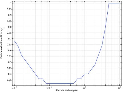
In the Settings window for 1D Plot Group, type Efficiency vs. Particle Radius in the Label text field.
|
|
3
|
|
4
|
|
5
|
|
6
|
Locate the Plot Settings section.
|
|
7
|
|
8
|
Select the y-axis label checkbox. In the associated text field, type Particle collection efficiency.
|
|
9
|
|
1
|
|
2
|
|
3
|
|
4
|
|
5
|
|
6
|
|
7
|
|
1
|
|
2
|
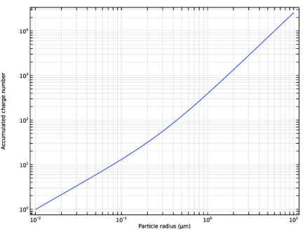
In the Settings window for 1D Plot Group, type Accumulated Charge Number vs. Particle Radius in the Label text field.
|
|
3
|
|
4
|
|
1
|
In the Model Builder window, expand the Accumulated Charge Number vs. Particle Radius node, then click Particle 1.
|
|
2
|
|
3
|
|
4
|