PDF

Electrodeless Lamp
Introduction
This model simulates an electrodeless lamp with argon/mercury chemistry. The low excitation threshold for mercury atoms means that even though the mercury is present in small concentrations, its interaction with electrons determines the overall discharge characteristics. here is strong UV emission from the plasma at 185 nm and 253 nm stemming from spontaneous decay of electronically excited mercury atoms. The UV emission can stimulate phosphors coated on the surface of the bulb resulting in visible light. From an electrical point of view, the lamp can be thought of as a transformer, where the coil acts as the primary and the plasma acts as the secondary. If the efficiency of discharge lamps could be increased by 1%, it would result in a saving of 109 kWh per year worldwide.
Note: This application requires the Plasma Module and the AC/DC Module.
Model Definition
A schematic of the geometry used to solve the problem is given in Figure 1. A sinusoidal current is applied to the copper coil (green) which creates a magnetic field in the ferrite core (gray). When the plasma ignites, a magnetic circuit is created between the ferrite core and the plasma. The free electrons in the plasma bulk are accelerated by the electric field. This leads to creation of new electrons through ionization which sustains the plasma. In quasi steady-state, the creation of new electrons is balanced by the loss of electrons to the wall.
Figure 1: Diagram of electrodeless light source.
The presence of mercury leads to the formation of electronically excited mercury atoms. Certain excited states emit a photon at a given wavelength with a certain emission frequency. By solving for the number density of each of the excited species, you can determine the amount of energy channeled into creating the excited mercury atoms. You can then calculate the amount of energy emitted from the plasma as photons.
In order to simplify the analysis, the following assumptions are made:
plasma chemistry
The chemical mechanism comes from Ref. 1 and consists of 11 species and 96 reactions. The electron impact cross-section data is obtained from Ref. 2, Ref. 3, Ref. 4, and Ref. 5
Ar++Hg=>Hg++Ar
Ar++Ar=>Ar+Ar+
Hg++Hg=>Hg+Hg+
The following surface reactions are considered:
Electron transport is modeled by solving the continuity equation, the momentum equation under the drift-diffusion approximation, and the mean electron energy equation (for detailed information on electron transport, see Theory for the Drift Diffusion Interface in the Plasma Module User’s Guide)
The source coefficients in the above equations are determined by the plasma chemistry. The electron rate expression is defined as
where νe,j is the stoichiometric coefficient, and the reaction rate is defined as
where kjf is the forward rate constant and kjr is the reversed rate constant. Both the Electron Impact Reaction feature and Reaction feature can contribute to the electron rate expression. However, when using the Reaction feature it is important to note that the associated electron energy gain or loss is not included in the source term of the electron mean energy equation.
The rate constants can be computed from electron impact cross-section data
where γ = (2q/me)1/2 (SI unit: C1/2/kg1/2), me is the electron mass (SI unit: kg), ε is the electron energy (SI unit: V), σ is the electron impact collision cross section (SI unit: m2), and f is the electron energy distribution function.
When Townsend coefficients are used, the reaction rate is defined as
where αj/Nn is the reduced Townsend coefficient for reaction j (SI unit: m2) and Γe is the electron flux as defined above (SI unit: 1/(m2·s)). Townsend coefficients can increase the stability of the numerical scheme when the electron flux is field driven as is the case with DC discharges.
The total electron energy loss or gained is calculated by summing the collisional energy changes from all reactions defined with the Electron Impact Reaction feature as
where Δεj is the energy loss from reaction j (SI unit: V) and F is the Faraday constant (SI unit: C/mol). For excitation and ionization collisions Δεj corresponds to the energy of the excited state being excited/deexcited or ionized, for attachment Δεj is set to zero, and for elastic collisions
where me and mk are the electron and heavy species mass in kg, Te is the electron temperature in eV, and Tgas is the gas temperature in K.
For heavy species, the following equation is solved for the mass fraction of each species (for detailed information on the transport of the nonelectron species, see Theory for the Heavy Species Transport Interface in the Plasma Module User’s Guide):
The electrostatic field is computed using the following equation:
The space charge density ρ is automatically computed based on the plasma chemistry specified in the model using the formula
For detailed information about electrostatics see Theory for the Electrostatics Interface in the Plasma Module User’s Guide.
For a nonmagnetized and nonpolarized plasma, the induction currents are computed in the frequency domain using the following equation:
The plasma conductivity needs to be specified as a material property, usually from the cold plasma approximation:
where ne is the electron density, q is the electron charge, me is the electron mass, νe is the collision frequency and ω is the angular frequency.
electrical excitation
The lamp is operated by a fixed power of 80 watts. This means that the total power dissipation in the system is 80 W. Some of the power is lost in the coil and the ferrite but the bulk of the power is channeled into the plasma.
Results and Discussion
The results are presented below.
Figure 2: Surface plot of electron density inside the column.
The electron density is plotted in Figure 2. The electron density is high, as one would expect in an inductively coupled plasma. The peak value of the electron density at the driving frequency used in the model results in a peak plasma conductivity of around 180 S/m. The high value for the electron density and low excitation and ionization threshold for mercury results in a very low electron “temperature” which is plotted in Figure 3. The peak electron temperature is only 1.27 eV, which through Boltzmann’s relation results in a low plasma potential. The plasma potential is plotted in Figure 4 and only peaks at 8 V.
Figure 3: Plot of the electron “temperature”.
Figure 4: Plot of plasma potential.
Figure 5: Plot of the resistive losses.
Figure 6: Plot of the mole fraction of ground state mercury.
Figure 7: Plot of the number density of mercury ions.
The resistive losses in the plasma are plotted in Figure 5. The plasma skin depth is a few centimeters so there is no real shielding of the azimuthal electric field. The mole fraction of the ground state mercury is plotted in Figure 6. The mole fraction is low in the core of the plasma and higher on the walls. This is because the electrons consume the ground state mercury in the plasma core, converting it to electronically excited states. The electronically excited mercury atoms diffuse to the walls of the lamp where they de-excite back to the ground state. This continuous consumption of ground state mercury in the plasma bulk and release on the walls results in large gradients in mole fraction within the bulb.
There are two ion species present in the plasma, argon, and mercury. Despite the fact that the number density of ground state argon is 25 times higher than mercury, the density of mercury ions is several hundred times greater than the density of argon ions. This is because the ionization energy for mercury is only 10.44 eV compared to 15.7 eV for argon. Direct ionization of mercury is preferable to argon because the tail of the electron energy distribution function drops dramatically at higher electron energies. Additionally, any argon ions which encounter a ground state or electronically excited mercury atom donate their charge because it is energetically favorable.
Figure 8: Plot of the mole fraction of Hg(63P1). Spontaneous decay of this species is responsible for the generation of 253 nm radiation.
The mole fraction of Hg(63P1) is plotted in Figure 8. These atoms spontaneously emit photos at a frequency factor of 8·106 s1. On the way to the walls of the lamp, the photons continuously excite mercury atoms and then be released when spontaneous decay occurs. This resonant absorption and reabsorption of the photons means that the frequency factor appears to be much lower than it actually is. Since a self-consistent model of the radiation imprisonment of the photons is computationally impractical, a trapping factor is used to approximate this effect. A trapping factor of 10 is used for the Hg(63P1) atoms which means that the frequency factor is lowered by a factor of 10. In Figure 9 the mole fraction of Hg(61P1) is plotted. A trapping factor of 1000 is used for the spontaneous decay back to ground state mercury.
Figure 9: Plot of the mole fraction of Hg(61P1). Spontaneous decay of this species is responsible for the generation of 185 nm radiation.
References
1. K. Rajaraman, Radiation Transport in Low Pressure Plasmas: Lighting and Semiconductor Etching Plasmas, PhD thesis, Depart. of Physics, University of Illinois, 2005.
2. Phelps database, www.lxcat.net, retrieve in 2017.
3. S.D. Rockwood, “Elastic and Inelastic Cross Sections for Electron-Hg Scattering from Hg Transport Data,” Phys. Rev. A, vol. 8, no. 5, pp. 2348–2358, 1973.
4. L. Vriens and A.H. Smeets, “Cross-section and Rate Formulas for Electron-impact Ionization, Excitation, Deexcitation, and Total Depopulation of Excited Atoms,” Phys. Rev. A, vol. 22, no. 3, pp. 940–951, 1980.
5. C. Kenty, “Production of 2537 Radiation and the Role of Metastable Atoms in an Argon-Mercury Discharges,” Journal of Applied Physics, vol. 21, pp. 1309–1318, 1950.
Application Library path: Plasma_Module/Inductively_Coupled_Plasmas/electrodeless_lamp
Modeling Instructions
From the File menu, choose New.
New
In the New window, click  Model Wizard.
Model Wizard
1
In the Model Wizard window, click  2D Axisymmetric.
2
In the Select Physics tree, select Plasma > Inductively Coupled Plasma.
3
Click Add.
4
Click  Study.
5
In the Select Study tree, select Preset Studies for Selected Multiphysics > Frequency–Transient.
6
Geometry 1
Line Segment 1 (ls1)
1
In the Geometry toolbar, click  More Primitives and choose Line Segment.
2
In the Settings window for Line Segment, locate the Starting Point section.
3
From the Specify list, choose Coordinates.
4
Locate the Endpoint section. From the Specify list, choose Coordinates.
5
In the r text field, type 0.015.
Cubic Bézier 1 (cb1)
1
In the Geometry toolbar, click  More Primitives and choose Cubic Bézier.
2
In the Settings window for Cubic Bézier, locate the Control Points section.
3
In row 1, set r to 0.015.
4
In row 2, set r to 0.015.
5
In row 3, set r to 0.03.
6
In row 4, set r to 0.03.
7
In row 2, set z to 0.025.
8
In row 3, set z to 0.025.
9
In row 4, set z to 0.045.
Quadratic Bézier 1 (qb1)
1
In the Geometry toolbar, click  More Primitives and choose Quadratic Bézier.
2
In the Settings window for Quadratic Bézier, locate the Control Points section.
3
In row 1, set r to 0.03.
4
In row 2, set r to 0.03.
5
In row 1, set z to 0.045.
6
In row 2, set z to 0.07.
7
In row 3, set z to 0.07.
Line Segment 2 (ls2)
1
In the Geometry toolbar, click  More Primitives and choose Line Segment.
2
In the Settings window for Line Segment, locate the Starting Point section.
3
From the Specify list, choose Coordinates.
4
Locate the Endpoint section. From the Specify list, choose Coordinates.
5
Locate the Starting Point section. In the z text field, type 0.07.
6
Click  Build All Objects.
Convert to Solid 1 (csol1)
1
In the Geometry toolbar, click  Conversions and choose Convert to Solid.
2
Click in the Graphics window and then press Ctrl+A to select all objects.
3
In the Settings window for Convert to Solid, click  Build All Objects.
Rectangle 1 (r1)
1
In the Geometry toolbar, click  Rectangle.
2
In the Settings window for Rectangle, locate the Size and Shape section.
3
In the Width text field, type 0.004.
4
In the Height text field, type 0.05.
Rectangle 2 (r2)
1
In the Geometry toolbar, click  Rectangle.
2
In the Settings window for Rectangle, locate the Size and Shape section.
3
In the Width text field, type 0.006.
4
In the Height text field, type 0.052.
Rectangle 3 (r3)
1
In the Geometry toolbar, click  Rectangle.
2
In the Settings window for Rectangle, locate the Size and Shape section.
3
In the Width text field, type 0.007.
4
In the Height text field, type 0.053.
Chamfer 1 (cha1)
1
In the Geometry toolbar, click  Chamfer.
2
Click the  Zoom Extents button in the Graphics toolbar.
3
Click the  Zoom In button in the Graphics toolbar.
4
On the object r2, select Point 3 only.
It might be easier to select the correct point by using the Selection List window. To open this window, in the Home toolbar click Windows and choose Selection List. (If you are running the cross-platform desktop, you find Windows in the main menu.)
5
In the Settings window for Chamfer, locate the Distance section.
6
In the Distance from vertex text field, type 1.5e-3.
7
Click  Build All Objects.
Chamfer 2 (cha2)
1
In the Geometry toolbar, click  Chamfer.
2
On the object r3, select Point 3 only.
3
In the Settings window for Chamfer, locate the Distance section.
4
In the Distance from vertex text field, type 2e-3.
5
Click  Build All Objects.
Square 1 (sq1)
1
In the Geometry toolbar, click  Square.
2
In the Settings window for Square, locate the Size section.
3
In the Side length text field, type 0.001.
4
Locate the Position section. In the r text field, type 0.0045.
5
In the z text field, type 0.025.
6
Click  Build All Objects.
Array 1 (arr1)
1
In the Geometry toolbar, click  Transforms and choose Array.
2
3
In the Settings window for Array, locate the Size section.
4
From the Array type list, choose Linear.
5
In the Size text field, type 5.
6
Locate the Displacement section. In the z text field, type 5e-3.
7
Click  Build All Objects.
8
Click the  Zoom Extents button in the Graphics toolbar.
Definitions
Variables 1
1
In the Definitions toolbar, click  Local Variables.
2
In the Settings window for Variables, locate the Variables section.
3
Coil boundaries
1
In the Definitions toolbar, click  Explicit.
2
3
In the Settings window for Explicit, locate the Output Entities section.
4
From the Output entities list, choose Adjacent boundaries.
5
In the Label text field, type Coil boundaries.
Coil domains
1
In the Definitions toolbar, click  Explicit.
2
3
In the Settings window for Explicit, type Coil domains in the Label text field.
Boundary layers
1
In the Definitions toolbar, click  Explicit.
2
In the Settings window for Explicit, locate the Input Entities section.
3
From the Geometric entity level list, choose Boundary.
4
5
In the Label text field, type Boundary layers.
Discharge
1
In the Definitions toolbar, click  Explicit.
2
3
In the Settings window for Explicit, type Discharge in the Label text field.
Since the molecular weights of the species are very different, activate the mixture diffusion correction.
Plasma (plas)
1
In the Model Builder window, under Component 1 (comp1) click Plasma (plas).
2
In the Settings window for Plasma, locate the Transport Settings section.
3
Select the Mixture diffusion correction checkbox.
4
The Plasma Chemistry Import feature
The next steps have instructions to use the Plasma Chemistry Import feature to import a file that automatically creates the argon-mercury plasma chemistry.
The following is set or created automatically:
a
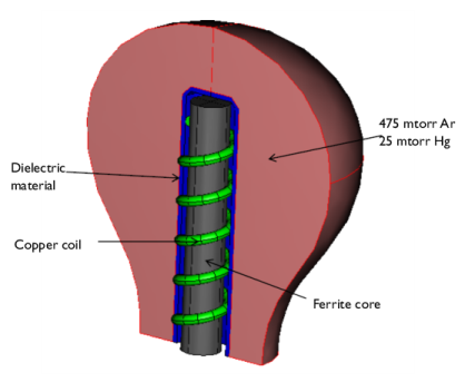
Species properties using User defined species data
b
c
The documentation accompanying the Plasma Chemistry Import feature contains more information about the file structure and what can be set automatically.
Plasma Chemistry Import 1
1
In the Physics toolbar, click  Global and choose Plasma Chemistry Import.
2
In the Settings window for Plasma Chemistry Import, locate the Plasma Chemistry Import section.
3
Click  Browse.
4
5
Click  Import.
The surface reactions used in the model were created automatically but it is still necessary to specify at which boundary they are going to exist.
Surface Reactions - Walls
1
In the Model Builder window, click Surface Reactions - Walls.
2
In the Settings window for Surface Reaction Group, locate the Boundary Selection section.
3
From the Selection list, choose Boundary layers.
Species: Hg
1
In the Model Builder window, expand the Component 1 (comp1) > Plasma (plas) > Group - Species node, then click Species: Hg.
2
In the Settings window for Species, locate the General Parameters section.
3
In the x0 text field, type 0.05.
Species: Hg1
1
In the Model Builder window, click Species: Hg1.
2
In the Settings window for Species, locate the General Parameters section.
3
In the x0 text field, type 2E-6.
Species: Hg2
1
In the Model Builder window, click Species: Hg2.
2
In the Settings window for Species, locate the General Parameters section.
3
In the x0 text field, type 1E-6.
Species: Hg3
1
In the Model Builder window, click Species: Hg3.
2
In the Settings window for Species, locate the General Parameters section.
3
In the x0 text field, type 5E-6.
Species: Hg4
1
In the Model Builder window, click Species: Hg4.
2
In the Settings window for Species, locate the General Parameters section.
3
In the x0 text field, type 1E-6.
Species: Hg5
1
In the Model Builder window, click Species: Hg5.
2
In the Settings window for Species, locate the General Parameters section.
3
In the x0 text field, type 5E-6.
Species: Hg6
1
In the Model Builder window, click Species: Hg6.
2
In the Settings window for Species, locate the General Parameters section.
3
In the x0 text field, type 1E-6.
Species: Ar
1
In the Model Builder window, click Species: Ar.
2
In the Settings window for Species, locate the Species Formula section.
3
Select the From mass constraint checkbox.
Species: Ar+
1
In the Model Builder window, click Species: Ar+.
2
In the Settings window for Species, locate the General Parameters section.
3
In the n0 text field, type 1E16.
Species: Hg+
1
In the Model Builder window, click Species: Hg+.
2
In the Settings window for Species, locate the Species Formula section.
3
Select the Initial value from electroneutrality constraint checkbox.
Group - Species
In the Model Builder window, collapse the Component 1 (comp1) > Plasma (plas) > Group - Species node.
Plasma Model 1
1
In the Model Builder window, click Plasma Model 1.
2
In the Settings window for Plasma Model, locate the Electron Density and Energy section.
3
From the Electron transport properties list, choose From electron impact reactions.
4
Locate the Model Inputs section. In the T text field, type Tinit.
5
In the pA text field, type pinit.
Ground 1
1
In the Physics toolbar, click  Boundaries and choose Ground.
2
In the Settings window for Ground, locate the Boundary Selection section.
3
From the Selection list, choose Boundary layers.
Wall 1
1
In the Physics toolbar, click  Boundaries and choose Wall.
2
In the Settings window for Wall, locate the Boundary Selection section.
3
From the Selection list, choose Boundary layers.
Initial Values 1
1
In the Model Builder window, click Initial Values 1.
2
In the Settings window for Initial Values, locate the Initial Values section.
3
In the ne,0 text field, type 1E17.
4
In the ε0 text field, type 2.
Magnetic Fields (mf)
In the Model Builder window, under Component 1 (comp1) click Magnetic Fields (mf).
Domain Coil 1
1
In the Physics toolbar, click  Domains and choose Domain Coil.
2
In the Settings window for Domain Coil, locate the Domain Selection section.
3
From the Selection list, choose Coil domains.
4
Locate the Coil section. Select the Coil group checkbox.
5
From the Coil excitation list, choose Power.
6
In the Pcoil text field, type lamp_power.
7
Click the  Zoom Extents button in the Graphics toolbar.
Materials
Coils
1
In the Model Builder window, under Component 1 (comp1) right-click Materials and choose Blank Material.
2
3
In the Settings window for Material, locate the Material Contents section.
4
5
In the Label text field, type Coils.
Ferrite
1
Right-click Materials and choose Blank Material.
2
3
In the Settings window for Material, locate the Material Contents section.
4
5
In the Label text field, type Ferrite.
Air
1
Right-click Materials and choose Blank Material.
2
3
In the Settings window for Material, locate the Material Contents section.
4
5
In the Label text field, type Air.
Dielectric
1
Right-click Materials and choose Blank Material.
2
3
In the Settings window for Material, locate the Material Contents section.
4
5
In the Label text field, type Dielectric.
Mesh 1
1
In the Model Builder window, under Component 1 (comp1) click Mesh 1.
2
In the Settings window for Mesh, locate the Physics-Controlled Mesh section.
3
From the Element size list, choose Extra fine.
Edge 1
1
In the Mesh toolbar, click  More Generators and choose Edge.
2
In the Settings window for Edge, locate the Boundary Selection section.
3
From the Selection list, choose Coil boundaries.
Distribution 1
1
Right-click Edge 1 and choose Distribution.
2
In the Settings window for Distribution, locate the Boundary Selection section.
3
From the Selection list, choose Coil boundaries.
4
Locate the Distribution section. From the Distribution type list, choose Predefined.
5
In the Number of elements text field, type 30.
6
In the Element ratio text field, type 6.
7
From the Growth rate list, choose Exponential.
8
Select the Symmetric distribution checkbox.
Mapped 1
1
In the Mesh toolbar, click  Mapped.
2
In the Settings window for Mapped, locate the Domain Selection section.
3
From the Geometric entity level list, choose Domain.
4
From the Selection list, choose Coil domains.
Edge 2
1
In the Mesh toolbar, click  More Generators and choose Edge.
2
Size 1
1
Right-click Edge 2 and choose Size.
2
In the Settings window for Size, locate the Element Size section.
3
Click the Custom button.
4
Locate the Element Size Parameters section.
5
Select the Maximum element size checkbox. In the associated text field, type 5e-4.
Edge 3
1
In the Mesh toolbar, click  More Generators and choose Edge.
2
Size 1
1
Right-click Edge 3 and choose Size.
2
In the Settings window for Size, locate the Element Size section.
3
Click the Custom button.
4
Locate the Element Size Parameters section.
5
Select the Maximum element size checkbox. In the associated text field, type 1e-3.
Boundary Layers 1
1
In the Mesh toolbar, click  Boundary Layers.
2
In the Settings window for Boundary Layers, locate the Domain Selection section.
3
From the Geometric entity level list, choose Domain.
4
5
Click to expand the Transition section. Clear the Smooth transition to interior mesh checkbox.
Boundary Layer Properties
1
In the Model Builder window, click Boundary Layer Properties.
2
In the Settings window for Boundary Layer Properties, locate the Boundary Selection section.
3
From the Selection list, choose Boundary layers.
4
Locate the Layers section. In the Stretching factor text field, type 1.1.
5
From the Thickness specification list, choose First layer.
6
In the Thickness text field, type 2E-5.
Free Triangular 1
1
In the Mesh toolbar, click  Free Triangular.
2
In the Settings window for Free Triangular, click  Build All.
Study 1
Step 1: Frequency–Transient
1
In the Model Builder window, under Study 1 click Step 1: Frequency–Transient.
2
In the Settings window for Frequency–Transient, locate the Study Settings section.
3
In the Frequency text field, type 2[MHz].
4
In the Output times text field, type 0.
5
Click  Range.
6
In the Range dialog, choose Number of values from the Entry method list.
7
In the Start text field, type -8.
8
In the Stop text field, type log10(2e-3).
9
In the Number of values text field, type 3.
10
From the Function to apply to all values list, choose exp10(x) – Exponential function (base 10).
11
Click Add.
12
In the Study toolbar, click  Compute.
Results
Power Deposition
1
In the Results toolbar, click  2D Plot Group.
2
In the Settings window for 2D Plot Group, type Power Deposition in the Label text field.
Surface 1
1
Right-click Power Deposition and choose Surface.
2
In the Settings window for Surface, click Replace Expression in the upper-right corner of the Expression section. From the menu, choose Component 1 (comp1) > Magnetic Fields > Heating and losses > mf.Qrh - Volumetric loss density, electric - W/m³.
3
Locate the Coloring and Style section. From the Color table list, choose ThermalWave.
Selection 1
1
Right-click Surface 1 and choose Selection.
2
3
In the Power Deposition toolbar, click  Plot.
Ground State Mercury Mole Fraction
1
In the Results toolbar, click  2D Plot Group.
2
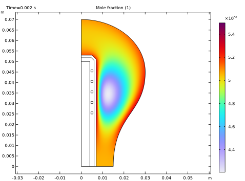
In the Settings window for 2D Plot Group, type Ground State Mercury Mole Fraction in the Label text field.
Surface 1
1
Right-click Ground State Mercury Mole Fraction and choose Surface.
2
In the Settings window for Surface, click Replace Expression in the upper-right corner of the Expression section. From the menu, choose Component 1 (comp1) > Plasma > Mole fractions > plas.x_wHg - Mole fraction - 1.
3
In the Ground State Mercury Mole Fraction toolbar, click  Plot.
Mercury Ion Number Density
1
In the Results toolbar, click  2D Plot Group.
2
In the Settings window for 2D Plot Group, type Mercury Ion Number Density in the Label text field.
Surface 1
1
Right-click Mercury Ion Number Density and choose Surface.
2
In the Settings window for Surface, click Replace Expression in the upper-right corner of the Expression section. From the menu, choose Component 1 (comp1) > Plasma > Number densities > plas.n_wHg_1p - Number density - 1/m³.
3
In the Mercury Ion Number Density toolbar, click  Plot.
Mole Fraction of Excited Mercury 2
1
In the Results toolbar, click  2D Plot Group.
2
In the Settings window for 2D Plot Group, type Mole Fraction of Excited Mercury 2 in the Label text field.
Surface 1
1
Right-click Mole Fraction of Excited Mercury 2 and choose Surface.
2
In the Settings window for Surface, click Replace Expression in the upper-right corner of the Expression section. From the menu, choose Component 1 (comp1) > Plasma > Mole fractions > plas.x_wHg2 - Mole fraction - 1.
3
In the Mole Fraction of Excited Mercury 2 toolbar, click  Plot.
Mole Fraction of Excited Mercury 4
1
In the Results toolbar, click  2D Plot Group.
2
In the Settings window for 2D Plot Group, type Mole Fraction of Excited Mercury 4 in the Label text field.
Surface 1
1
Right-click Mole Fraction of Excited Mercury 4 and choose Surface.
2
In the Settings window for Surface, click Replace Expression in the upper-right corner of the Expression section. From the menu, choose Component 1 (comp1) > Plasma > Mole fractions > plas.x_wHg4 - Mole fraction - 1.
3
In the Mole Fraction of Excited Mercury 4 toolbar, click  Plot.