PDF

Global Model of a CF4/O2 Plasma Reactor for Silicon Etching
Introduction
This tutorial studies the etching of silicon using a CF4/O2 plasma using a global model. The plasma and surface chemistries are based on Ref. 1 and Ref. 2, and the electron impact reactions are taken from LxCat (Ref. 3, Ref. 4, and Ref. 5).
Model Definition
The model used in this work assumes that the spatial distribution of the different quantities in the plasma reactor can be treated as uniform. Without spatial derivatives, the numerical solution of the equation set becomes considerably simpler and the computation time is reduced. These advantages make a global model a good first approach to study a plasma reactor, especially when complex chemistries are involved.
When using a global plasma model the species densities and the electron temperature are treated as volume-averaged quantities. Detailed information on the global model can be found in the section Theory for Global Models in the Plasma Module User’s Guide. For heavy species the following equation is solved for the mass fraction
where ρ is the mass density (SI unit: kg/m3), wk is the mass fraction, wf,k is the mass fraction in the feed, mf and mo are the mass-flow rates of the total feed and outlet, and Rk is the rate expression (SI unit: kg/(m3·s)). The fourth term on the right-hand side accounts for surface losses and creation, where Al is the surface area, hl is a dimensionless correction term, V is the reactor volume, Mk is the species molar mass (SI unit: kg/mol) and Rsurf,k,l is the surface rate expression (SI unit: mol/(m2·s)) at a surface l. The last term is introduced because the species mass balance equations are written in the nonconservative form and it used the mass-continuity equation to replace for the mass density time derivative. In the last term Mf,l is the inward mass flux of surface l (SI unit: kg/(m2·s)). The sum in the last two terms is over all surfaces where there are surface reactions.
To take possible variations of the system’s total mass or pressure into account, the mass-continuity equation can also be solved:
.
The electron number density is obtained from electroneutrality:
Using the local energy approximation (LEA), the electron energy density nε (SI unit: V/ m3) is computed from
where Rε is the electron energy loss due to inelastic and elastic collisions, Pabs is the power absorbed by the electrons (SI unit: W), and e is the elementary charge. The last term on the right side accounts for the kinetic energy transported to the surface by electrons and ions. The summation is over all positive ions, εe is the mean kinetic energy lost per electron lost, εi is the mean kinetic energy lost per ion lost, and Na is Avogadro’s number. If using the local field approximation (LFA) the electron mean energy equation is not solved and the electron mean energy can be: (i) provided as a function of the electric field; or (ii) obtained by solving the Boltzmann equation in the two-term approximation.
The rate coefficients for electron impact reactions can be computed by appropriate averaging of cross sections over an EEDF. The EEDF can either be analytic or obtained by solving the steady-state Boltzmann equation in the two-term approximation coupled with the equation system (The Boltzmann Equation, Two-Term Approximation Interface in the Plasma Module User’s Guide). When solving for the EEDF, the coupling between the equations is as follows: (i) if the LEA is used, the electron mean energy obtained from the electron mean energy equation is given as input to the Boltzmann solver; (ii) if the LFA is used, the reduced electric field must be given as input to the Boltzmann solver and the electron mean energy comes from averaging over the computed EEDF.
This model uses the LEA and a Maxwellian EEDF, as in Ref. 1.
Plasma Chemistry
The plasma chemistry is based on Ref. 1 and Ref. 2. The electron impact cross sections used in this model are retrieved from different databases from LxCat: Ref. 3, Ref. 4, and Ref. 5. The data from Ref. 3 further refers to Ref. 6 and Ref. 7. The model solves for 29 volume species: electrons, CF4, CF3, CF2, CF, CF3+, CF2+, CF+, F2, F2+, F, F+, F-, O2, O2+, O, O+,O-O, O2*, O*, C, C+, CO2, CO2+, CO, CO+, COF, COF2, and FO.
The enchant products in the gaseous phase Si, SiF, SiF2, SiF3, and SiF4 are assumed not to influence the plasma discharge. Reactions with these species are not included and these species are not solved for.
The following surface species are also included: Si(s), SiF(s), SiF2(s), and SiF3(s). The model solves for the site fraction of each species and Si(s) is set to be the empty site species. The empty site species is not solved for and its site fraction is obtained from the total site constraint.
When modeling surface species with a stationary solver, one of the surface species needs to be specified as an empty site species to be computed from a surface site constraint.
In this model, the etching process begins with fluorine atom adsorption at surface sites (Table 1) followed by chemical etching, which is negligible under the current conditions (Table 2), and ion-enhanced etching and sputtering (Table 3).
I++Si(s)=>I+Si
I++SiF(s)=>I+SiF
I++SiF2(s)=>I+SiF2
I++SiF3(s)=>I+SiF3
In Table 3, I+ denotes an ion that becomes neutralized upon reaching the surface and removes surface species into the gas phase, with a specified yield that depends on the ion energy. In the present model, the ion energy is treated as a parameter.
When explicitly solving for surface sites, rather than using a generic reaction to represent wall interactions, it is necessary to specify all possible reactions involving the available surface sites. For example, a generic wall recombination might be written as F=>0.5F2, but in a surface-site-based formulation, this process is represented as shown in Table 4.
Results and Discussion
The model contains two studies. In the first study, a base case is solved using a time-dependent solver for an input power of 200 W, pressure of 350 mTorr, and an oxygen mole fraction (xO2) of 0.01. In the second study, the oxygen mole fraction is varied between 0.01 and 0.8 for 15, 25, and 50 V of ion energy. The ion energy is assumed to be the same for all ion and is only used to compute the yield of ion enhanced etching reactions.
The etching rate of Si (ESi) is define by the flux of Si containing species from the surface, ΓESi = ΓSi + ΓSiF + ΓSiF2 + ΓSiF3 + ΓSiF4, divided by the density of Si, nSi = 5.0 × 1028 m3:
.
In the plasma interface, fluxes at surfaces are defined by Rsurf variables. For an individual Surface Reaction feature defined as F+Si(s)=>Si+F the flux of Si at the surface is defined by the variable plas.Rsurf_#_Si_surf, where # is the reaction number. In a Surface Reaction Group the flux of a given species at the surface is defined by the variable plas.Rsurf_srg#_SpeciesName_surf, where # is the Surface Reaction Group number. This variable sums over all reactions involving that species. In the present model all surface reactions that cause removal of Si from the surface (except chemical etching that is negligible for the present conditions) are grouped in a Surface Reaction Group labeled as “Waffer - Ion Enhance Etching and Sputtering”. This way, the flux of Si containing species used to compute etching can be computed by the sum of the variables plas.Rsurf_srg5_Si_surf, plas.Rsurf_srg5_SiF_surf, plas.Rsurf_srg5_SiF2_surf, and plas.Rsurf_srg5_SiF3_surf.
Figure 1 shows the etching rate as a function of the F number density (nF) for several ion energies. Three regimes are observed in agreement with Ref. 8 (page 584) where a detailed explanation is provided. Here, only the key points are summarized. In the first regime (up to about 15% of xO2) both ESi and nF increase with xO2. This is explained by the “burning” of CFx species creating F atoms. In the second regime (from 15% to 40% of xO2) ESi starts to decrease with xO2 even if nF continues to increase. Ref. 8 explains this trend as the result of competition of O atoms in surface sites SiFx(s). However, in the present model, such surface mechanisms are not included and that might explain why the etching rate variation is smaller in this regime. We could say that in the present model the second regime described in Ref. 8 is absent and what is observed is a direct transition to the third regime where both ESi and nF decrease with xO2, which is believed to be due to oxygen dilution.
Figure 1: Silicon etching rate as a function of atomic fluorine number density at ion energies of 10, 25, and 50 V. The color scale represents the mole fraction of oxygen.
References
1. T. Kimura and M. Noto, “Experimental study and global model of inductively coupled CF4/O2 discharges,” J. Appl. Phys., vol. 100, no. 063303, pp. 1–9, 2006; doi.org/10.1063/1.2345461.
2. P. Ho, J.E. Johannes, R.J. Buss, and E. Meeks, “Chemical Reaction Mechanisms for Modeling the Fluorocarbon Plasma Etch of Silicon Oxide and Related Materials,” Sandia Report SAND2001-1292, 2001; doi.org/10.2172/782704
3. Bordage database, www.lxcat.net, retrieved on 2025.
4. Morgan database, www.lxcat.net, retrieved on 2025.
5. Phelps database, www.lxcat.net, retrieved 2025.
6. M.C. Bordage, P. Segur, and A. Chouki, “Determination of a set of electron impact cross sections in tetrafluoromethane consistent with experimental determination of swarm parameters,” J. Appl. Phys., vol. 80, no. 3, p. 1325–1336, 1996; doi.org/10.1063/1.362931.
7. M.C. Bordage, P. Segur, L.G. Christophorou, and J.K. Olthoff, “Boltzmann analysis of electron swarm parameters in CF4 using independently assessed electron-collision cross sections,” J. Appl. Phys., vol. 86, no. 7, pp. 3558–3566, 1999; doi.org/10.1063/1.371258.
8. M.A. Lieberman and A.J. Lichtenberg, Principles of Plasma Discharges and Materials Processing, John Wiley & Sons, 2025.
Application Library path: Plasma_Module/Surface_Processing/cf4_o2_si_etching_global_model
Modeling Instructions
From the File menu, choose New.
New
In the New window, click  Model Wizard.
Model Wizard
1
In the Model Wizard window, click  2D Axisymmetric.
2
In the Select Physics tree, select Plasma > Plasma (plas).
3
Click Add.
4
Click  Study.
5
In the Select Study tree, select General Studies > Time Dependent.
6
Global Definitions
Parameters 1
Add some parameters to be used in the model.
1
In the Model Builder window, under Global Definitions click Parameters 1.
2
In the Settings window for Parameters, locate the Parameters section.
3
Click  Load from File.
4
Set the domain dimensions. The volume and surface areas used in the global model of the reactor are obtained automatically from this geometry.
Geometry 1
1
In the Model Builder window, under Component 1 (comp1) click Geometry 1.
2
In the Settings window for Geometry, locate the Units section.
3
From the Length unit list, choose cm.
Rectangle 1 (r1)
1
In the Geometry toolbar, click  Rectangle.
2
In the Settings window for Rectangle, locate the Size and Shape section.
3
In the Width text field, type R0.
4
In the Height text field, type L0.
Plasma (plas)
Choose to solve for a global model of a constant pressure reactor.
1
In the Model Builder window, under Component 1 (comp1) click Plasma (plas).
2
In the Settings window for Plasma, locate the Diffusion Model section.
3
From the Diffusion model list, choose Global.
4
Locate the Plasma Properties section. Select the Use reduced electron transport properties checkbox.
5
Locate the Reactor section. From the Reactor type list, choose Constant pressure.
Plasma Model 1
Set the pressure, mass flow, power absorbed by the electrons, and an estimation of the plasma sheath voltage drop (for the mean kinetic energy lost per ion lost).
1
In the Model Builder window, under Component 1 (comp1) > Plasma (plas) click Plasma Model 1.
2
In the Settings window for Plasma Model, locate the Model Inputs section.
3
In the T text field, type Tgas.
4
In the pA text field, type p0.
5
Locate the Total Mass Flow section. In the Qsccm text field, type Qfeed.
6
Locate the Mean Electron Energy Specification section. In the Pabs text field, type pw.
7
In the εe text field, type 2*plas.Te.
8
In the εi text field, type Vp.
The Plasma Chemistry Import feature
The next steps show how to use the Plasma Chemistry Import feature to import a file that automatically creates the CF4/O2 plasma chemistry.
The following is set or created automatically:
a
b
c
The documentation accompanying the Plasma Chemistry Import feature contains more information about the file structure and what can be set automatically.
Plasma Chemistry Import 1
1
In the Physics toolbar, click  Global and choose Plasma Chemistry Import.
2
In the Settings window for Plasma Chemistry Import, locate the Plasma Chemistry Import section.
3
Click  Browse.
4
5
Click  Import.
Set some properties of the species and the surface reactions.
Set CF4 to be the species for which the mass fraction is found from the mass constraint.
Set the feed mole fraction for CF4 and O2.
Species: CF4
1
In the Model Builder window, expand the Component 1 (comp1) > Plasma (plas) > Group - Species node, then click Species: CF4.
2
In the Settings window for Species, locate the Species Formula section.
3
Select the From mass constraint checkbox.
4
Locate the General Parameters section. In the xfeed text field, type 1-xO2.
Species: O2
1
In the Model Builder window, click Species: O2.
2
In the Settings window for Species, locate the General Parameters section.
3
In the xfeed text field, type xO2.
This model assumes that etchant products do not influence the discharge. To not solve for the etchant products in the gaseous phase, use a Species Constraint Group species to constrain their densities to their initial values.
Species Constraint Group 1
1
In the Physics toolbar, click  Domains and choose Species Constraint Group.
2
3
In the Settings window for Species Constraint Group, locate the Species Group section.
4
5
6
7
8
9
10
11
12
13
In the following, select the boundaries for each of the Surface Reaction Group features.
Group - Species
In the Model Builder window, collapse the Component 1 (comp1) > Plasma (plas) > Group - Species node.
Surface Reactions - Side Walls
1
In the Model Builder window, click Surface Reactions - Side Walls.
2
Surface Reactions - Wafer - Adsorption, Chemical Etching, and Recombination
1
In the Model Builder window, click Surface Reactions - Wafer - Adsorption, Chemical Etching, and Recombination.
2
Surface Reactions - Wafer - Lumped
1
In the Model Builder window, click Surface Reactions - Wafer - Lumped.
2
Surface Reactions - Wafer Radical Abstraction
1
In the Model Builder window, click Surface Reactions - Wafer Radical Abstraction.
2
Surface Reactions - Wafer - Ion Enhanced Etching and Sputtering
1
In the Model Builder window, click Surface Reactions - Wafer - Ion Enhanced Etching and Sputtering.
2
Select Si(s) to be identified as an empty site species. This way, the site fraction for Si(s) is not solved for. Instead, it is obtained from total site conservation.
Species: Si(s)
1
In the Model Builder window, expand the Component 1 (comp1) > Plasma (plas) > Group - Surface Species node, then click Species: Si(s).
2
In the Settings window for Surface Species, locate the Species Formula section.
3
Select the Empty site species checkbox.
Use a time-dependent solver to provide good initial conditions for a subsequent stationary solver where parameterizations are made.
Base Case
1
In the Model Builder window, click Study 1.
2
In the Settings window for Study, type Base Case in the Label text field.
3
Locate the Study Settings section. Clear the Generate default plots checkbox.
Step 1: Time Dependent
1
In the Model Builder window, under Base Case click Step 1: Time Dependent.
2
In the Settings window for Time Dependent, locate the Study Settings section.
3
In the Output times text field, type 10^{range(log10(1.0e-7),1/2,log10(50))}.
4
In the Study toolbar, click  Compute.
Add a stationary study to parameterize the O2 mole fraction and ion energy.
Since the solution from a previous study is used to provide initial conditions and solutions from previous steps are reused, it is possible to increase the initial damping factor to 1. This will reduce the computation time.
Add Study
1
In the Home toolbar, click  Add Study to open the Add Study window.
2
Go to the Add Study window.
3
Find the Studies subsection. In the Select Study tree, select General Studies > Stationary.
4
Click the Add Study button in the window toolbar.
5
In the Home toolbar, click  Add Study to close the Add Study window.
Study 2
Step 1: Stationary
1
In the Settings window for Stationary, click to expand the Values of Dependent Variables section.
2
Find the Initial values of variables solved for subsection. From the Settings list, choose User controlled.
3
From the Method list, choose Solution.
4
From the Study list, choose Base Case, Time Dependent.
5
From the Time (s) list, choose Last.
6
In the Model Builder window, click Study 2.
7
In the Settings window for Study, locate the Study Settings section.
8
Clear the Generate default plots checkbox.
Solution 2 (sol2)
1
In the Study toolbar, click  Show Default Solver.
2
In the Model Builder window, expand the Solution 2 (sol2) node.
3
In the Model Builder window, expand the Study 2 > Solver Configurations > Solution 2 (sol2) > Stationary Solver 1 node, then click Fully Coupled 1.
4
In the Settings window for Fully Coupled, click to expand the Method and Termination section.
5
In the Initial damping factor text field, type 1.
Parametric Sweep
1
In the Study toolbar, click  Parametric Sweep.
2
In the Settings window for Parametric Sweep, locate the Study Settings section.
3
4
5
6
7
From the Sweep type list, choose All combinations.
8
Click to expand the Advanced Settings section. Select the Reuse solution from previous step checkbox.
9
In the Study toolbar, click  Compute.
Results
Create plots to show the electron density, electron temperature, electronegativity, species number density, site fraction, and etching rate.
Electron Density
1
In the Results toolbar, click  1D Plot Group.
2
In the Settings window for 1D Plot Group, type Electron Density in the Label text field.
3
Locate the Data section. From the Dataset list, choose Study 2/Solution 2 (sol2).
4
Click to expand the Title section. From the Title type list, choose None.
5
Locate the Legend section. From the Position list, choose Upper left.
Global 1
1
Right-click Electron Density and choose Global.
2
In the Settings window for Global, locate the y-Axis Data section.
3
4
Click to expand the Legends section. Find the Include subsection. Clear the Description checkbox.
5
In the Electron Density toolbar, click  Plot.
Electron Temperature
1
In the Model Builder window, right-click Electron Density and choose Duplicate.
2
In the Settings window for 1D Plot Group, type Electron Temperature in the Label text field.
Global 1
1
In the Model Builder window, expand the Electron Temperature node, then click Global 1.
2
In the Settings window for Global, locate the y-Axis Data section.
3
4
In the Electron Temperature toolbar, click  Plot.
Electron Temperature
1
In the Model Builder window, click Electron Temperature.
2
In the Settings window for 1D Plot Group, locate the Legend section.
3
From the Position list, choose Upper right.
Electronegativity
1
Right-click Electron Temperature and choose Duplicate.
2
In the Settings window for 1D Plot Group, type Electronegativity in the Label text field.
Global 1
1
In the Model Builder window, expand the Electronegativity node, then click Global 1.
2
In the Settings window for Global, locate the y-Axis Data section.
3
4
In the Electronegativity toolbar, click  Plot.
Neutral Species Number Density
1
In the Results toolbar, click  1D Plot Group.
2
In the Settings window for 1D Plot Group, type Neutral Species Number Density in the Label text field.
3
Locate the Title section. From the Title type list, choose None.
4
Locate the Plot Settings section.
5
Select the y-axis label checkbox. In the associated text field, type Number density (1/m<sup>3</sup>).
6
Locate the Legend section. From the Position list, choose Lower right.
Global 1
1
Right-click Neutral Species Number Density and choose Global.
2
In the Settings window for Global, locate the y-Axis Data section.
3
Neutral Species Number Density
1
In the Model Builder window, click Neutral Species Number Density.
2
In the Settings window for 1D Plot Group, locate the Data section.
3
From the Dataset list, choose Study 2/Solution 2 (sol2).
4
From the Parameter selection (Eion) list, choose Last.
5
Locate the Axis section. Select the y-axis log scale checkbox.
Global 1
1
In the Model Builder window, click Global 1.
2
In the Settings window for Global, locate the Legends section.
3
Find the Include subsection. Clear the Solution checkbox.
4
In the Neutral Species Number Density toolbar, click  Plot.
Charged Species Number Density
1
In the Model Builder window, right-click Neutral Species Number Density and choose Duplicate.
2
In the Settings window for 1D Plot Group, type Charged Species Number Density in the Label text field.
Global 1
1
In the Model Builder window, expand the Charged Species Number Density node, then click Global 1.
2
In the Settings window for Global, locate the y-Axis Data section.
3
Click  Clear Table.
4
5
In the Charged Species Number Density toolbar, click  Plot.
Site Fraction
1
In the Results toolbar, click  1D Plot Group.
2
In the Settings window for 1D Plot Group, type Site Fraction in the Label text field.
3
Locate the Data section. From the Dataset list, choose Study 2/Solution 2 (sol2).
4
From the Parameter selection (Eion) list, choose Last.
5
Locate the Title section. From the Title type list, choose None.
6
Locate the Plot Settings section.
7
Select the y-axis label checkbox. In the associated text field, type Site fraction (1).
Global 1
1
Right-click Site Fraction and choose Global.
2
In the Settings window for Global, locate the y-Axis Data section.
3
4
Locate the Legends section. Find the Include subsection. Clear the Solution checkbox.
5
In the Site Fraction toolbar, click  Plot.
Etching Rate vs. F Number Density
1
In the Results toolbar, click  1D Plot Group.
2
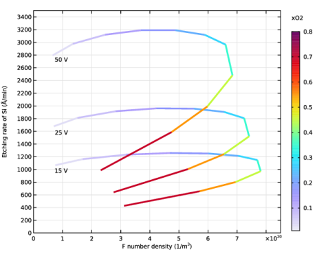
In the Settings window for 1D Plot Group, type Etching Rate vs. F Number Density in the Label text field.
3
Locate the Title section. From the Title type list, choose None.
4
Locate the Data section. From the Dataset list, choose Study 2/Solution 2 (sol2).
5
From the Parameter selection (Eion) list, choose From list.
6
In the Parameter values (Eion (V)) list box, select 15.
Global 1
1
Right-click Etching Rate vs. F Number Density and choose Global.
2
In the Settings window for Global, locate the y-Axis Data section.
3
4
Locate the x-Axis Data section. From the Parameter list, choose Expression.
5
In the Expression text field, type plas.n_wF.
6
Click to expand the Coloring and Style section. From the Width list, choose 3.
7
Locate the Legends section. Clear the Show legends checkbox.
Color Expression 1
1
Right-click Global 1 and choose Color Expression.
2
In the Settings window for Color Expression, locate the Expression section.
3
In the Expression text field, type xO2.
4
In the Etching Rate vs. F Number Density toolbar, click  Plot.
Global 2
1
In the Model Builder window, under Results > Etching Rate vs. F Number Density right-click Global 1 and choose Duplicate.
2
In the Settings window for Global, locate the Data section.
3
From the Dataset list, choose Study 2/Solution 2 (sol2).
4
From the Parameter selection (Eion) list, choose From list.
5
In the Parameter values (Eion (V)) list box, select 25.
6
In the Etching Rate vs. F Number Density toolbar, click  Plot.
Color Expression 1
1
In the Model Builder window, expand the Global 2 node, then click Color Expression 1.
2
In the Settings window for Color Expression, locate the Coloring and Style section.
3
Clear the Color legend checkbox.
Global 3
1
In the Model Builder window, under Results > Etching Rate vs. F Number Density right-click Global 2 and choose Duplicate.
2
In the Settings window for Global, locate the Data section.
3
In the Parameter values (Eion (V)) list box, select 50.
4
In the Etching Rate vs. F Number Density toolbar, click  Plot.
Etching Rate vs. F Number Density
1
In the Model Builder window, click Etching Rate vs. F Number Density.
2
In the Settings window for 1D Plot Group, locate the Color Legend section.
3
Select the Show titles checkbox.
4
Locate the Axis section. Select the Manual axis limits checkbox.
5
In the x minimum text field, type 0.
6
In the x maximum text field, type 8.5e20.
7
In the y minimum text field, type 0.
8
In the y maximum text field, type 3500.
9
In the Etching Rate vs. F Number Density toolbar, click  Plot.
Annotation 1
1
Right-click Etching Rate vs. F Number Density and choose Annotation.
2
In the Settings window for Annotation, locate the Annotation section.
3
In the Text text field, type 50 V.
4
Locate the Position section. In the R text field, type 0.6e20.
5
In the Z text field, type 2800.
6
Locate the Coloring and Style section. Clear the Show point checkbox.
Annotation 2
1
Right-click Annotation 1 and choose Duplicate.
2
In the Settings window for Annotation, locate the Position section.
3
In the Z text field, type 1650.
4
Locate the Annotation section. In the Text text field, type 25 V.
Annotation 3
1
Right-click Annotation 2 and choose Duplicate.
2
In the Settings window for Annotation, locate the Position section.
3
In the Z text field, type 1050.
4
Locate the Annotation section. In the Text text field, type 15 V.
Color Expression 1
1
In the Model Builder window, under Results > Etching Rate vs. F Number Density > Global 1 click Color Expression 1.
2
In the Settings window for Color Expression, locate the Coloring and Style section.
3
In the Color legend title text field, type xO2.
Etching Rate vs. F Number Density
1
In the Model Builder window, under Results click Etching Rate vs. F Number Density.
2
In the Settings window for 1D Plot Group, locate the Plot Settings section.
3
Select the x-axis label checkbox. In the associated text field, type F number density (1/m<sup>3</sup>).
4
Select the y-axis label checkbox. In the associated text field, type Etching rate of Si (Å/min).
5
In the Etching Rate vs. F Number Density toolbar, click  Plot.