PDF

Global Model of a CF4/O2 Plasma Reactor
Introduction
This tutorial studies the plasma chemistry of a CF4/O2 plasma at low pressure using a global model. The plasma chemistry is based on Ref. 1 and the electron impact reactions are taken from LxCat (Ref. 2, Ref. 3, and Ref. 4).
Model Definition
The model used in this work assumes that the spatial distribution of the different quantities in the plasma reactor can be treated as uniform. Without spatial derivatives, the numerical solution of the equation set becomes considerably simpler and the computation time is reduced. These advantages make a global model a good first approach to study a plasma reactor, especially when complex chemistries are involved.
When using a global plasma model the species densities and the electron temperature are treated as volume-averaged quantities. Detailed information on the global model can be found in the section Theory for Global Models in the Plasma Module User’s Guide. For heavy species the following equation is solved for the mass fraction
where ρ is the mass density (SI unit: kg/m3), wk is the mass fraction, wf,k is the mass fraction in the feed, mf and mo are the mass-flow rates of the total feed and outlet, and Rk is the rate expression (SI unit: kg/(m3·s)). The fourth term on the right-hand side accounts for surface losses and creation, where Al is the surface area, hl is a dimensionless correction term, V is the reactor volume, Mk is the species molar mass (SI unit: kg/mol) and Rsurf,k,l is the surface rate expression (SI unit: mol/(m2·s)) at a surface l. The last term is introduced because the species mass balance equations are written in the nonconservative form and it used the mass-continuity equation to replace for the mass density time derivative. In the last term Mf,l is the inward mass flux of surface l (SI unit: kg/(m2·s)). The sum in the last two terms is over all surfaces where there are surface reactions.
To take possible variations of the system’s total mass or pressure into account, the mass-continuity equation can also be solved:
.
The electron number density is obtained from electroneutrality:
Using the local energy approximation (LEA), the electron energy density nε (SI unit: V/ m3) is computed from
where Rε is the electron energy loss due to inelastic and elastic collisions, Pabs is the power absorbed by the electrons (SI unit: W), and e is the elementary charge. The last term on the right side accounts for the kinetic energy transported to the surface by electrons and ions. The summation is over all positive ions, εe is the mean kinetic energy lost per electron lost, εi is the mean kinetic energy lost per ion lost, and Na is Avogadro’s number. If using the local field approximation (LFA) the electron mean energy equation is not solved and the electron mean energy can be: (i) provided as a function of the electric field; or (ii) obtained by solving the Boltzmann equation in the two-term approximation.
The rate coefficients for electron impact reactions can be computed by appropriate averaging of cross sections over an EEDF. The EEDF can either be analytic or obtained by solving the steady-state Boltzmann equation in the two-term approximation coupled with the equation system (The Boltzmann Equation, Two-Term Approximation Interface in the Plasma Module User’s Guide). When solving for the EEDF, the coupling between the equations is as follows: (i) if the LEA is used, the electron mean energy obtained from the electron mean energy equation is given as input to the Boltzmann solver; (ii) if the LFA is used, the reduced electric field must be given as input to the Boltzmann solver and the electron mean energy comes from averaging over the computed EEDF.
This model uses the LEA and a Maxwellian EEDF, as in Ref. 1.
Plasma Chemistry
The plasma chemistry is based on Ref. 1. The electron impact cross sections used in this model are retrieved from different databases from LxCat: Ref. 2, Ref. 3, and Ref. 4. The data from Ref. 2 further refers to Ref. 5 and Ref. 6. The model includes 29 species: electrons, CF4, CF3, CF2, CF, CF3+, CF2+, CF+, F2, F2+, F, F+, F-, O2, O2+, O, O+, O-, O2*, O*, C, C+, CO2, CO2+, CO, CO+, COF, COF2, and FO.
Results and Discussion
The model contains two studies. In the first study, a base case is solved using a time-dependent solver for an input power of 120 W and an oxygen mole fraction of 0.01. In the second study, the power is kept at 120 W and the oxygen mole fraction is varied between 0 and 1 for pressures of 8, 15, and 25 mTorr.
Figure 1, Figure 2, Figure 3, and Figure 4 show the electron density, electron temperature, F number density, and O number density, respectively. In general, there is good agreement with the results from Ref. 1.
Figure 1: Electron number density as a function of oxygen mole fraction for several pressures.
Figure 2: Electron temperature as a function of oxygen mole fraction for several pressures.
Figure 3: F number density as a function of oxygen mole fraction for several pressures.
Figure 4: O number density as a function of oxygen mole fraction for several pressures.
References
1. T. Kimura and M. Noto, “Experimental study and global model of inductively coupled CF4/O2 discharges,” J. Appl. Phys., vol. 100, no. 063303, pp. 1–9, 2006; doi.org/10.1063/1.2345461.
2. Bordage database, www.lxcat.net, retrieved on 2025.
3. Morgan database, www.lxcat.net, retrieved on 2025.
4. Phelps database, www.lxcat.net, retrieved 2025.
5. M.C. Bordage, P. Segur, and A. Chouki, “Determination of a set of electron impact cross sections in tetrafluoromethane consistent with experimental determination of swarm parameters,” J. Appl. Phys., vol. 80, no. 3, p. 1325–1336, 1996; doi.org/10.1063/1.362931.
6. M.C. Bordage, P. Segur, L.G. Christophorou, and J.K. Olthoff, “Boltzmann analysis of electron swarm parameters in CF4 using independently assessed electron-collision cross sections,” J. Appl. Phys., vol. 86, no. 7, pp. 3558–3566, 1999; doi.org/10.1063/1.371258.
Application Library path: Plasma_Module/Global_Modeling/cf4_o2_global_model
Modeling Instructions
From the File menu, choose New.
New
In the New window, click  Model Wizard.
Model Wizard
1
In the Model Wizard window, click  2D Axisymmetric.
2
In the Select Physics tree, select Plasma > Plasma (plas).
3
Click Add.
4
Click  Study.
5
In the Select Study tree, select General Studies > Time Dependent.
6
Global Definitions
Parameters 1
Add some parameters to be used in the model.
1
In the Model Builder window, under Global Definitions click Parameters 1.
2
In the Settings window for Parameters, locate the Parameters section.
3
Click  Load from File.
4
Set the domain dimensions. The volume and surface areas used in the global model of the reactor are obtained automatically from this geometry.
Geometry 1
1
In the Model Builder window, under Component 1 (comp1) click Geometry 1.
2
In the Settings window for Geometry, locate the Units section.
3
From the Length unit list, choose cm.
Rectangle 1 (r1)
1
In the Geometry toolbar, click  Rectangle.
2
In the Settings window for Rectangle, locate the Size and Shape section.
3
In the Width text field, type R0.
4
In the Height text field, type L0.
Plasma (plas)
Choose to solve for a global model of a constant pressure reactor.
1
In the Model Builder window, under Component 1 (comp1) click Plasma (plas).
2
In the Settings window for Plasma, locate the Diffusion Model section.
3
From the Diffusion model list, choose Global.
4
Locate the Plasma Properties section. Select the Use reduced electron transport properties checkbox.
5
Locate the Reactor section. From the Reactor type list, choose Constant pressure.
Plasma Model 1
Set the pressure, mass flow, power absorbed by the electrons, and an estimation of the plasma sheath voltage drop (for the mean kinetic energy lost per ion lost).
1
In the Model Builder window, under Component 1 (comp1) > Plasma (plas) click Plasma Model 1.
2
In the Settings window for Plasma Model, locate the Model Inputs section.
3
In the T text field, type Tgas.
4
In the pA text field, type p0.
5
Locate the Total Mass Flow section. In the Qsccm text field, type Qfeed.
6
Locate the Mean Electron Energy Specification section. In the Pabs text field, type pw.
7
In the εe text field, type 2*plas.Te.
8
In the εi text field, type Vp.
The Plasma Chemistry Import Feature
The next steps show how to use the Plasma Chemistry Import feature to import a file that automatically creates the CF4/O2 plasma chemistry.
The following is set or created automatically:
a
b
c
The documentation accompanying the Plasma Chemistry Import feature contains more information about the file structure and what can be set automatically.
Plasma Chemistry Import 1
1
In the Physics toolbar, click  Global and choose Plasma Chemistry Import.
2
In the Settings window for Plasma Chemistry Import, locate the Plasma Chemistry Import section.
3
Click  Browse.
4
5
Click  Import.
Set some properties of the species and the surface reactions.
Set CF4 to be the species for which the mass fraction is found from a mass constraint.
Set the feed mole fraction for CF4 and O2.
Species: CF4
1
In the Model Builder window, expand the Component 1 (comp1) > Plasma (plas) > Group - Species node, then click Species: CF4.
2
In the Settings window for Species, locate the Species Formula section.
3
Select the From mass constraint checkbox.
4
Locate the General Parameters section. In the xfeed text field, type 1-xO2.
Species: O2
1
In the Model Builder window, click Species: O2.
2
In the Settings window for Species, locate the General Parameters section.
3
In the xfeed text field, type xO2.
Plasma (plas)
Group - Species
In the Model Builder window, collapse the Component 1 (comp1) > Plasma (plas) > Group - Species node.
Surface Reactions - All Surfaces
1
In the Model Builder window, click Surface Reactions - All Surfaces.
2
In the Settings window for Surface Reaction Group, locate the Boundary Selection section.
3
From the Selection list, choose All boundaries.
Next, use a time-dependent study to find a solution for the base case. The solution from this study will provide initial conditions for a second study that sweeps for pressure and oxygen mole fraction.
Base Case
1
In the Model Builder window, click Study 1.
2
In the Settings window for Study, locate the Study Settings section.
3
Clear the Generate default plots checkbox.
4
In the Study toolbar, click  Compute.
5
In the Label text field, type Base Case.
Add Study
1
In the Home toolbar, click  Add Study to open the Add Study window.
2
Go to the Add Study window.
3
Find the Studies subsection. In the Select Study tree, select General Studies > Stationary.
4
Click the Add Study button in the window toolbar.
5
In the Home toolbar, click  Add Study to close the Add Study window.
Study 2
Step 1: Stationary
1
In the Settings window for Stationary, click to expand the Values of Dependent Variables section.
2
Find the Initial values of variables solved for subsection. From the Settings list, choose User controlled.
3
From the Method list, choose Solution.
4
From the Study list, choose Base Case, Time Dependent.
5
From the Time (s) list, choose Last.
6
Click to expand the Study Extensions section. Select the Auxiliary sweep checkbox.
7
From the Sweep type list, choose All combinations.
8
9
10
11
12
13
Click  Range.
14
In the Range dialog, type 0.01 in the Start text field.
15
In the Step text field, type 0.1.
16
In the Stop text field, type 0.95.
17
Click Replace.
18
In the Settings window for Stationary, locate the Study Extensions section.
19
From the Reuse solution from previous step list, choose Yes.
Since you already have a solution from a previous study and are reusing the solution from the previous step, you can set the initial damping factor to 1.
Solution 2 (sol2)
1
In the Study toolbar, click  Show Default Solver.
2
In the Model Builder window, expand the Solution 2 (sol2) node.
3
In the Model Builder window, expand the Study 2 > Solver Configurations > Solution 2 (sol2) > Stationary Solver 1 node, then click Fully Coupled 1.
4
In the Settings window for Fully Coupled, click to expand the Method and Termination section.
5
In the Initial damping factor text field, type 1.
6
In the Model Builder window, click Study 2.
7
In the Settings window for Study, type xO2 and Pressure Sweep in the Label text field.
8
Locate the Study Settings section. Clear the Generate default plots checkbox.
9
In the Study toolbar, click  Compute.
Results
Create plots to show the electron density, electron temperature, F number density, and O number density.
Electron Density
1
In the Results toolbar, click  1D Plot Group.
2
In the Settings window for 1D Plot Group, type Electron Density in the Label text field.
3
Locate the Data section. From the Dataset list, choose xO2 and Pressure Sweep/Solution 2 (sol2).
4
Click to expand the Title section. From the Title type list, choose None.
Global 1
1
Right-click Electron Density and choose Global.
2
In the Settings window for Global, locate the y-Axis Data section.
3
4
Locate the Data section. From the Dataset list, choose xO2 and Pressure Sweep/Solution 2 (sol2).
5
From the Parameter selection (p0) list, choose From list.
6
In the Parameter values (p0 (mTorr)) list box, select 8.
7
Click to expand the Legends section. Find the Include subsection. Clear the Description checkbox.
8
In the Electron Density toolbar, click  Plot.
Global 2
1
Right-click Global 1 and choose Duplicate.
2
In the Settings window for Global, locate the Data section.
3
In the Parameter values (p0 (mTorr)) list box, select 15.
4
In the Electron Density toolbar, click  Plot.
Global 3
1
Right-click Global 2 and choose Duplicate.
2
In the Settings window for Global, locate the Data section.
3
In the Parameter values (p0 (mTorr)) list box, select 25.
4
In the Electron Density toolbar, click  Plot.
Electron Density
1
In the Model Builder window, click Electron Density.
2
In the Settings window for 1D Plot Group, locate the Axis section.
3
Select the Manual axis limits checkbox.
4
In the y minimum text field, type 1e16.
5
In the y maximum text field, type 3e17.
6
In the Electron Density toolbar, click  Plot.
7
Select the y-axis log scale checkbox.
Electron Temperature
1
Right-click Electron Density and choose Duplicate.
2
In the Settings window for 1D Plot Group, type Electron Temperature in the Label text field.
Global 1
1
In the Model Builder window, expand the Electron Temperature node, then click Global 1.
2
In the Settings window for Global, locate the y-Axis Data section.
3
Global 2
1
In the Model Builder window, click Global 2.
2
In the Settings window for Global, locate the y-Axis Data section.
3
Global 3
1
In the Model Builder window, click Global 3.
2
In the Settings window for Global, locate the y-Axis Data section.
3
4
In the Electron Temperature toolbar, click  Plot.
Electron Temperature
1
In the Model Builder window, click Electron Temperature.
2
In the Settings window for 1D Plot Group, locate the Axis section.
3
Clear the y-axis log scale checkbox.
4
In the y minimum text field, type 0.
5
In the y maximum text field, type 5.
6
In the Electron Temperature toolbar, click  Plot.
F Density
1
Right-click Electron Temperature and choose Duplicate.
2
In the Settings window for 1D Plot Group, type F Density in the Label text field.
Global 1
1
In the Model Builder window, expand the F Density node, then click Global 1.
2
In the Settings window for Global, locate the y-Axis Data section.
3
Global 2
1
In the Model Builder window, click Global 2.
2
In the Settings window for Global, locate the y-Axis Data section.
3
Global 3
1
In the Model Builder window, click Global 3.
2
In the Settings window for Global, locate the y-Axis Data section.
3
F Density
1
In the Model Builder window, click F Density.
2
In the Settings window for 1D Plot Group, locate the Plot Settings section.
3
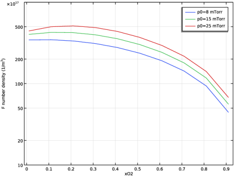
Select the y-axis label checkbox. In the associated text field, type F number density (1/m<sup>3</sup>).
4
Locate the Axis section. Select the y-axis log scale checkbox.
5
In the y minimum text field, type 1e18.
6
In the y maximum text field, type 1e20.
7
In the F Density toolbar, click  Plot.
O Density
1
Right-click F Density and choose Duplicate.
2
In the Settings window for 1D Plot Group, type O Density in the Label text field.
Global 1
1
In the Model Builder window, expand the O Density node, then click Global 1.
2
In the Settings window for Global, locate the y-Axis Data section.
3
Global 2
1
In the Model Builder window, click Global 2.
2
In the Settings window for Global, locate the y-Axis Data section.
3
Global 3
1
In the Model Builder window, click Global 3.
2
In the Settings window for Global, locate the y-Axis Data section.
3
O Density
1
In the Model Builder window, click O Density.
2
In the Settings window for 1D Plot Group, locate the Plot Settings section.
3
In the y-axis label text field, type O number density (1/m<sup>3</sup>).
4
Locate the Axis section. In the y maximum text field, type 1e21.
5
In the O Density toolbar, click  Plot.