PDF

Benchmark Model of a Capacitively Coupled Plasma
Introduction
The underlying physics of a capacitively coupled plasma is rather complicated, even for rather simple geometric configurations and plasma chemistries. This model benchmarks the Plasma, Time Periodic interface against many different codes, the results of which are taken from Ref. 1.
Model Definition
The model geometry consists of a 1D gap of 0.067 m. A plasma forms in the gap provided the driving voltage and fill pressure are high enough. The driving frequency in this model is 13.56 MHz. Helium chemistry is used, as was the case in Ref. 1.
Electron transport is modeled by solving the continuity equation, the momentum equation under the drift-diffusion approximation, and the mean electron energy equation (for detailed information on electron transport, see Theory for the Drift Diffusion Interface in the Plasma Module User’s Guide)
The source coefficients in the above equations are determined by the plasma chemistry. The electron rate expression is defined as
where νe,j is the stoichiometric coefficient, and the reaction rate is defined as
where kjf is the forward rate constant and kjr is the reversed rate constant. Both the Electron Impact Reaction feature and Reaction feature can contribute to the electron rate expression. However, when using the Reaction feature it is important to note that the associated electron energy gain or loss is not included in the source term of the electron mean energy equation.
The rate constants can be computed from electron impact cross-section data
where γ = (2q/me)1/2 (SI unit: C1/2/kg1/2), me is the electron mass (SI unit: kg), ε is the electron energy (SI unit: V), σ is the electron impact collision cross section (SI unit: m2), and f is the electron energy distribution function.
When Townsend coefficients are used, the reaction rate is defined as
where αj/Nn is the reduced Townsend coefficient for reaction j (SI unit: m2) and Γe is the electron flux as defined above (SI unit: 1/(m2·s)). Townsend coefficients can increase the stability of the numerical scheme when the electron flux is field driven as is the case with DC discharges.
The total electron energy loss or gained is calculated by summing the collisional energy changes from all reactions defined with the Electron Impact Reaction feature as
where Δεj is the energy loss from reaction j (SI unit: V) and F is the Faraday constant (SI unit: C/mol). For excitation and ionization collisions Δεj corresponds to the energy of the excited state being excited/deexcited or ionized, for attachment Δεj is set to zero, and for elastic collisions
where me and mk are the electron and heavy species mass in kg, Te is the electron temperature in eV, and Tgas is the gas temperature in K.
For heavy species, the following equation is solved for the mass fraction of each species (for detailed information on the transport of the nonelectron species, see Theory for the Heavy Species Transport Interface in the Plasma Module User’s Guide):
The electrostatic field is computed using the following equation:
The space charge density ρ is automatically computed based on the plasma chemistry specified in the model using the formula
For detailed information about electrostatics see Theory for the Electrostatics Interface in the Plasma Module User’s Guide.
In Ref. 1 the ion diffusivity is defined as:
and the mobility, μ as:
where a = qE/m and λ is the charge exchange mean free path. The same ion mobility and diffusivity models can be set in COMSOL. With that objective, choose Specify mobility, compute diffusivity and Use local field approximation in the section Mobility and Diffusivity Expressions on the ion species node. After that, go to the Mobility Specification and choose the High field ion mobility model with a Cross section σ equal to 3.1019 m2 to reproduce the same ion mobility and diffusivity as in Ref. 1.
boundary conditions
Electrons are lost to the wall due to random motion within a few mean free paths of the wall and gained due to secondary emission effects, resulting in the following boundary condition for the electron flux
(1)
and the electron energy flux
(2)
In order to make the COMSOL Multiphysics implementation of the electron losses to the wall consistent with the reference, the value of r must be set to 5/11. The second term on the right-hand side of Equation 1 is the gain of electrons due to secondary emission effects, γp being the secondary emission coefficient. The second term in Equation 2 is the secondary emission energy flux, εp being the mean energy of the secondary electrons. For the helium ions are lost to the wall due to surface reactions and the fact that the electric field is directed toward the wall:
Plasma Chemistry
The reference paper suggests a simplistic plasma chemistry for helium consisting of only 3 reactions and 4 species (electron impact cross sections are obtained from Ref. 2):
In addition to volumetric reactions, the following surface reactions are implemented:
When a metastable helium atom makes contact with the wall, it reverts to the ground state helium atom with some probability (the sticking coefficient).
Results and Discussion
The time averaged ion current density is plotted in Figure 1. The peak ion current density occurs on the electrodes, at a value of around 0.2 A/m2. At lower pressures the ion current density profile is more smooth across the gap. At 300 mtorr there is a pronounced flattening off of the ion current density in the plasma sheath. These results agree well with those presented in Figure 9 of Ref. 1.
Figure 1: Plot of the period averaged ion current as a function of the distance from the left electrode.
The period averaged excitation and ionization rates are plotted in Figure 2 and Figure 3.
Figure 2: Plot of the period averaged ionization rate as a function of the distance from the left electrode.
Figure 3: Plot of the period averaged excitation rate as a function of the distance from the left electrode.
The results for the ionization and excitation rates agree well with Ref. 1 in both absolute value and spatial distribution. The period averaged electron power deposition is plotted in Figure 4. The COMSOL results are again, in good agreement with the reference paper.
Figure 4: Plot of the period averaged electron power deposition as a function of the distance from the left electrode.
Figure 5 and Figure 6 plot the period averaged electron and ion density at different operating pressures. The electron and ion density is the same in the plasma bulk but the ion density is higher in the plasma sheath. This creates a net positive space charge density in the plasma sheath which tends to hold electrons in the plasma and accelerate ions toward the wall via the plasma potential.
Figure 5: Plot of the period averaged electron density at different operating pressures.
Figure 6: Plot of the period averaged ion density for different operating pressures.
Ref. 1 tabulates a wide range of lumped parameters for the discharge. These same parameters for the COMSOL model are shown in Table 3. There is good agreement between the COMSOL model and the values quoted in Ref. 1.
References
1. M. Surendra, “Radiofrequency discharge benchmark model comparison,” Plasma Sources Sci. Technol., vol. 4, pp 56–73, 1995.
2. Phelps database, www.lxcat.net, retrieved 2017.
Application Library path: Plasma_Module/Capacitively_Coupled_Plasmas/ccp_benchmark
Modeling Instructions
From the File menu, choose New.
New
In the New window, click  Model Wizard.
Model Wizard
1
In the Model Wizard window, click  1D.
2
In the Select Physics tree, select Plasma > Plasma, Time Periodic (ptp).
3
Click Add.
4
Click  Study.
5
In the Select Study tree, select Preset Studies for Selected Physics Interfaces > Time Periodic.
6
Start by drawing the geometry, which is simply a line of length 0.067m.
Geometry 1
Interval 1 (i1)
1
In the Model Builder window, under Component 1 (comp1) right-click Geometry 1 and choose Interval.
2
In the Settings window for Interval, locate the Interval section.
3
Define a parameter for the pressure, which will be used when sweeping over pressure in the study.
4
Click  Build All Objects.
Global Definitions
Parameters 1
1
In the Model Builder window, under Global Definitions click Parameters 1.
2
In the Settings window for Parameters, locate the Parameters section.
3
Define an expression for the input power. The expression is designed to obtain the same current density of 1 mA/cm^2 for each value of pressure.
Definitions (comp1)
Variables 1
1
In the Model Builder window, under Component 1 (comp1) right-click Definitions and choose Variables.
2
In the Settings window for Variables, locate the Variables section.
3
Turn off the source stabilization, since it is not needed in this example. Use the Fick’s law diffusion model to be consistent with the reference.
Plasma, Time Periodic (ptp)
1
In the Model Builder window, under Component 1 (comp1) click Plasma, Time Periodic (ptp).
2
In the Settings window for Plasma, Time Periodic, locate the Cross-Section Area section.
3
In the A text field, type 0.1[m^2].
4
Locate the Electron Energy Distribution Function Settings section. From the Electron energy distribution function list, choose Maxwellian.
5
Locate the Diffusion Model section. From the Diffusion model list, choose Fick’s law.
Cross Section Import 1
1
In the Physics toolbar, click  Global and choose Cross Section Import.
2
In the Settings window for Cross Section Import, locate the Cross Section Import section.
3
Click  Browse.
4
5
Click  Import.
Species: He
1
In the Model Builder window, click Species: He.
2
In the Settings window for Species, locate the Species Formula section.
3
Select the From mass constraint checkbox.
4
Locate the General Parameters section. From the Preset species data list, choose He.
Species: Hes
1
In the Model Builder window, click Species: Hes.
2
In the Settings window for Species, locate the General Parameters section.
3
From the Preset species data list, choose He.
4
In the Df text field, type 0.8[m^2/s].
Load in a table for the helium reduced ion mobility as a function of the reduced electric field. This table corresponds to the high field limit described in the reference.
Species: He+
1
In the Model Builder window, click Species: He+.
2
In the Settings window for Species, locate the Species Formula section.
3
Select the Initial value from electroneutrality constraint checkbox.
4
Locate the General Parameters section. From the Preset species data list, choose He.
5
Locate the Mobility and Diffusivity Expressions section. From the Specification list, choose Specify mobility, compute diffusivity.
6
From the Ion temperature list, choose Use local field approximation.
7
Locate the Mobility Specification section. From the Specify using list, choose Lookup table.
8
From the Mobility a function of list, choose Reduced electric field.
9
Find the Reduced ion mobility subsection. Click  Load from File.
10
Surface Reaction 1
1
In the Physics toolbar, click  Boundaries and choose Surface Reaction.
2
In the Settings window for Surface Reaction, locate the Reaction Formula section.
3
In the Formula text field, type He+=>He.
4
Locate the Boundary Selection section. From the Selection list, choose All boundaries.
5
Locate the Reaction Parameters section. In the γf text field, type 0.
6
Locate the Secondary Emission Parameters section. In the γi text field, type 0.
7
In the εi text field, type 0.
2: He+=>He
1
Right-click 1: He+=>He and choose Duplicate.
2
In the Settings window for Surface Reaction, locate the Reaction Formula section.
3
In the Formula text field, type Hes=>He.
4
Locate the Reaction Parameters section. In the γf text field, type 1.
Plasma Model 1
1
In the Model Builder window, click Plasma Model 1.
2
In the Settings window for Plasma Model, locate the Model Inputs section.
3
In the T text field, type 300[K].
4
In the pA text field, type p0.
5
Locate the Electron Density and Energy section. From the Electron transport properties list, choose Specify mobility only.
6
In the μe text field, type 3.33e24[1/(V*m*s)]/ptp.Nn.
Wall 1
1
In the Physics toolbar, click  Boundaries and choose Wall.
2
In the Settings window for Wall, locate the Boundary Selection section.
3
From the Selection list, choose All boundaries.
4
Locate the General Wall Settings section. In the re text field, type 5/11.
Ground 1
1
In the Physics toolbar, click  Boundaries and choose Ground.
2
Metal Contact 1
1
In the Physics toolbar, click  Boundaries and choose Metal Contact.
2
In the Settings window for Metal Contact, locate the Terminal section.
3
From the Source list, choose RF.
4
5
Locate the RF Source section. In the Prf text field, type Pin.
Mesh 1
Edge 1
In the Mesh toolbar, click  Edge.
Distribution 1
1
Right-click Edge 1 and choose Distribution.
2
In the Settings window for Distribution, locate the Distribution section.
3
From the Distribution type list, choose Predefined.
4
In the Number of elements text field, type 150.
5
In the Element ratio text field, type 10.
6
From the Growth rate list, choose Exponential.
7
Select the Symmetric distribution checkbox.
8
Click  Build All.
Study 1
Step 1: Time Periodic
1
In the Model Builder window, under Study 1 click Step 1: Time Periodic.
2
In the Settings window for Time Periodic, click to expand the Study Extensions section.
3
Select the Auxiliary sweep checkbox.
4
5
6
In the Model Builder window, click Study 1.
7
In the Settings window for Study, locate the Study Settings section.
8
Clear the Generate convergence plots checkbox.
9
Clear the Generate default plots checkbox.
10
In the Study toolbar, click  Compute.
Results
Create some plots to compare with the reference.
1D Plot Group 1
In the Results toolbar, click  1D Plot Group.
We need to use a built in operator to average over the extra dimension. This allows us to plot period averaged quantities for any variable.
Line Graph 1
1
Right-click 1D Plot Group 1 and choose Line Graph.
2
In the Settings window for Line Graph, locate the Selection section.
3
From the Selection list, choose All domains.
4
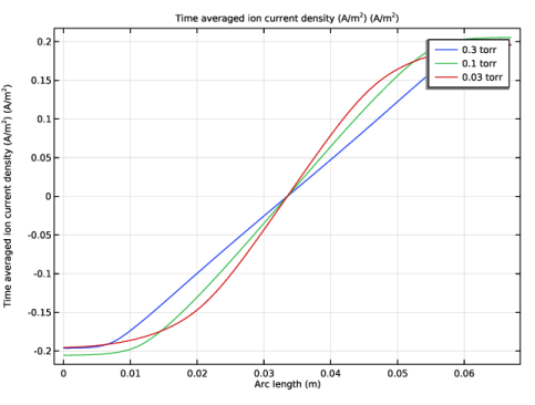
Locate the y-Axis Data section. In the Expression text field, type ptp.xdintop_ptp1(ptp.Jix_wHe_1p/ptp.xdim).
5
Click to expand the Quality section. From the Evaluation settings list, choose Manual.
6
From the Resolution list, choose No refinement.
7
Locate the y-Axis Data section.
8
Select the Description checkbox. In the associated text field, type Time averaged ion current density (A/m<sup>2</sup>).
9
Click to expand the Legends section. Select the Show legends checkbox.
10
In the 1D Plot Group 1 toolbar, click  Plot.
Time Averaged Ion Current Density
1
In the Model Builder window, under Results click 1D Plot Group 1.
2
In the Settings window for 1D Plot Group, type Time Averaged Ion Current Density in the Label text field.
3
In the Time Averaged Ion Current Density toolbar, click  Plot.
4
Click the  Zoom Extents button in the Graphics toolbar.
Time Averaged Ionization Rate
1
Right-click Time Averaged Ion Current Density and choose Duplicate.
2
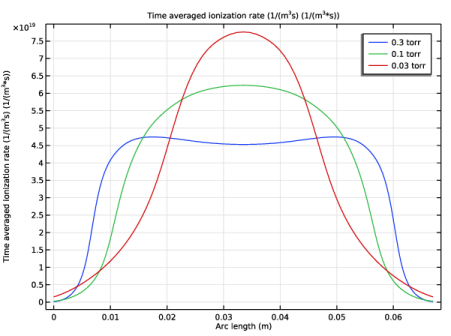
In the Settings window for 1D Plot Group, type Time Averaged Ionization Rate in the Label text field.
Line Graph 1
1
In the Model Builder window, expand the Time Averaged Ionization Rate node, then click Line Graph 1.
2
In the Settings window for Line Graph, locate the y-Axis Data section.
3
In the Expression text field, type ptp.Re_av.
4
In the Description text field, type Time averaged ionization rate (1/(m<sup>3</sup>s).
5
In the Time Averaged Ionization Rate toolbar, click  Plot.
6
Click the  Zoom Extents button in the Graphics toolbar.
Time Averaged Excitation Rate
1
In the Model Builder window, right-click Time Averaged Ionization Rate and choose Duplicate.
2
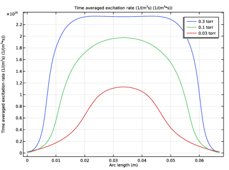
In the Settings window for 1D Plot Group, type Time Averaged Excitation Rate in the Label text field.
Line Graph 1
1
In the Model Builder window, expand the Time Averaged Excitation Rate node, then click Line Graph 1.
2
In the Settings window for Line Graph, locate the y-Axis Data section.
3
In the Expression text field, type ptp.xdintop_ptp1(ptp.R_wHes*N_A_const/ptp.xdim).
4
In the Description text field, type Time averaged excitation rate (1/(m<sup>3</sup>s).
5
In the Time Averaged Excitation Rate toolbar, click  Plot.
6
Click the  Zoom Extents button in the Graphics toolbar.
Time Averaged Electron Power Deposition
1
In the Model Builder window, right-click Time Averaged Excitation Rate and choose Duplicate.
2
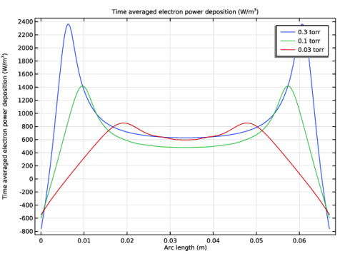
In the Settings window for 1D Plot Group, type Time Averaged Electron Power Deposition in the Label text field.
Line Graph 1
1
In the Model Builder window, expand the Time Averaged Electron Power Deposition node, then click Line Graph 1.
2
In the Settings window for Line Graph, locate the y-Axis Data section.
3
In the Expression text field, type ptp.Pcap_ele_ions_av-ptp.Pcap_ions_av.
4
In the Description text field, type Time averaged electron power deposition.
5
In the Time Averaged Electron Power Deposition toolbar, click  Plot.
6
Click the  Zoom Extents button in the Graphics toolbar.
7
In the Time Averaged Electron Power Deposition toolbar, click  Plot.
Time Averaged Electron Density
1
In the Model Builder window, right-click Time Averaged Electron Power Deposition and choose Duplicate.
2
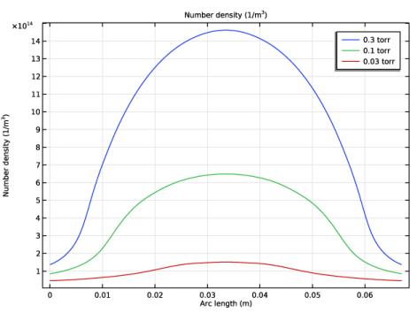
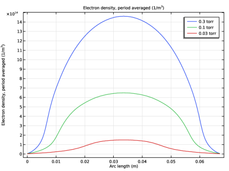
In the Settings window for 1D Plot Group, type Time Averaged Electron Density in the Label text field.
Line Graph 1
1
In the Model Builder window, expand the Time Averaged Electron Density node, then click Line Graph 1.
2
In the Settings window for Line Graph, click Replace Expression in the upper-right corner of the y-Axis Data section. From the menu, choose Component 1 (comp1) > Plasma, Time Periodic > Electron density > ptp.neav - Electron density, period averaged - 1/m³.
3
Locate the y-Axis Data section. Clear the Description checkbox.
4
In the Time Averaged Electron Density toolbar, click  Plot.
5
Click the  Zoom Extents button in the Graphics toolbar.
Time Averaged Ion Density
1
In the Model Builder window, right-click Time Averaged Electron Density and choose Duplicate.
2
In the Settings window for 1D Plot Group, type Time Averaged Ion Density in the Label text field.
Line Graph 1
1
In the Model Builder window, expand the Time Averaged Ion Density node, then click Line Graph 1.
2
In the Settings window for Line Graph, click Replace Expression in the upper-right corner of the y-Axis Data section. From the menu, choose Component 1 (comp1) > Plasma, Time Periodic > Number densities > ptp.n_wHe_1p_av - Number density - 1/m³.
3
In the Time Averaged Ion Density toolbar, click  Plot.
4
Click the  Zoom Extents button in the Graphics toolbar.
Study 1/Solution 1 (2) (sol1)
1
In the Model Builder window, expand the Results > Datasets node.
2
Right-click Results > Datasets > Study 1/Solution 1 (sol1) and choose Duplicate.
3
In the Settings window for Solution, locate the Solution section.
4
From the Component list, choose Extra Dimension from Plasma, Time Periodic (ptp_xdim).
Electric Potential
1
In the Results toolbar, click  1D Plot Group.
2
In the Settings window for 1D Plot Group, locate the Data section.
3
From the Dataset list, choose Study 1/Solution 1 (2) (sol1).
4
In the Label text field, type Electric Potential.
Line Graph 1
1
Right-click Electric Potential and choose Line Graph.
2
In the Settings window for Line Graph, locate the Selection section.
3
From the Selection list, choose All domains.
4
Click Replace Expression in the upper-right corner of the y-Axis Data section. From the menu, choose Component 1 (comp1) > Plasma, Time Periodic > Metal Contact 1 > ptp.mct1.V - Electric potential - V.
5
Locate the Legends section. Select the Show legends checkbox.
6
In the Electric Potential toolbar, click  Plot.
7
Click the  Zoom Extents button in the Graphics toolbar.
Cut Point 1D 1
1
In the Results toolbar, click  More Datasets and choose Cut Point 1D.
2
In the Settings window for Cut Point 1D, locate the Point Data section.
3
In the X text field, type 0.067/2.
Point Evaluation 1
1
In the Model Builder window, under Results right-click Derived Values and choose Point Evaluation.
2
In the Settings window for Point Evaluation, locate the Data section.
3
From the Dataset list, choose Cut Point 1D 1.
4
Click Replace Expression in the upper-right corner of the Expressions section. From the menu, choose Component 1 (comp1) > Plasma, Time Periodic > Electron density > ptp.neav - Electron density, period averaged - 1/m³.
5
Locate the Expressions section. In the table, enter the following settings:
6
Click  Evaluate.
Line Average 1
1
In the Results toolbar, click  More Derived Values and choose Average > Line Average.
2
In the Settings window for Line Average, locate the Data section.
3
From the Dataset list, choose Study 1/Solution 1 (2) (sol1).
4
Locate the Selection section. From the Selection list, choose All domains.
5
Locate the Expressions section. In the table, enter the following settings:
6
Clicknext to  Evaluate, then choose Table 1 - Point Evaluation 1.