
|
|
|
|
1
|
In the Model Wizard window, Select the Boltzmann Equation, Two-Term Approximation (be) interface and the Mean Energies study.
|
|
2
|
click
|
|
3
|
|
4
|
Click Add.
|
|
5
|
Click
|
|
6
|
|
7
|
Click
|
|
1
|
In the Model Builder window, under Component 1 (comp1) click Boltzmann Equation, Two-Term Approximation (be).
|
|
2
|
In the Settings window for Boltzmann Equation, Two-Term Approximation, locate the Electron Energy Distribution Function Settings section.
|
|
3
|
From the Electron energy distribution function list, choose Boltzmann equation, two-term approximation (quadratic).
|
|
4
|
Select the Electron–electron collisions checkbox.
|
|
5
|
|
6
|
|
7
|
Select the Compute maximum energy checkbox.
|
|
1
|
|
2
|
|
3
|
Click
|
|
5
|
Click
|
|
1
|
|
2
|
|
3
|
|
5
|
Locate the Results section. Find the Generate the following default plots subsection. Clear the Mean electron energy checkbox.
|
|
6
|
Clear the Rate coefficients checkbox.
|
|
7
|
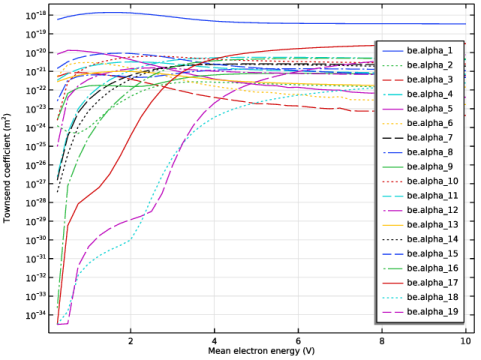
Select the Townsend coefficients checkbox.
|
|
8
|
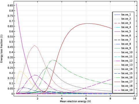
Select the Energy loss fraction checkbox.
|
|
1
|
|
2
|
|
3
|
|
1
|
|
2
|
|
3
|
Click
|
|
4
|
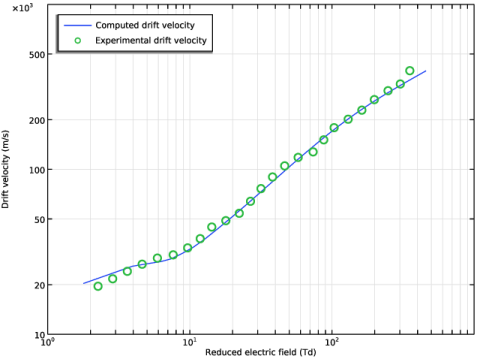
Browse to the model’s Application Libraries folder and double-click the file O2_drift_velocity_expt.txt.
|
|
5
|
|
6
|
In the Function table, enter the following settings:
|
|
1
|
|
2
|
|
3
|
Click
|
|
5
|
|
6
|
In the Function table, enter the following settings:
|
|
7
|
|
1
|
|
2
|
|
3
|
Click
|
|
4
|
|
5
|
|
6
|
|
7
|
Click Replace.
|
|
1
|
|
2
|
|
1
|
|
2
|
|
3
|
|
4
|
|
5
|
|
6
|
|
7
|
|
8
|
|
9
|
|
1
|
|
2
|
|
1
|
|
2
|
|
3
|
|
4
|
|
5
|
Select the Expression checkbox.
|
|
6
|
|
1
|
|
2
|
|
3
|
|
4
|
|
5
|
|
6
|
Select the Expression checkbox.
|
|
7
|
|
1
|
|
2
|
|
3
|
|
4
|
|
5
|
Locate the Plot Settings section.
|
|
6
|
|
7
|
|
8
|
|
9
|
|
10
|
|
11
|
|
12
|
|
13
|
Select the x-axis log scale checkbox.
|
|
14
|
Select the y-axis log scale checkbox.
|
|
15
|
|
1
|
|
2
|
|
4
|
|
5
|
|
6
|
|
1
|
|
2
|
|
4
|
|
5
|
|
6
|
|
7
|
Locate the Coloring and Style section. Find the Line style subsection. From the Line list, choose None.
|
|
8
|
|
9
|
|
10
|
|
11
|
|
12
|
|
1
|
|
2
|
|
3
|
|
4
|
|
5
|
Locate the Plot Settings section.
|
|
6
|
|
7
|
|
8
|
|
9
|
|
10
|
|
11
|
|
12
|
|
13
|
Select the x-axis log scale checkbox.
|
|
14
|
Select the y-axis log scale checkbox.
|
|
15
|
|
1
|
|
2
|
|
4
|
|
5
|
|
6
|
|
1
|
|
2
|
|
4
|
|
5
|
|
6
|
|
7
|
Locate the Coloring and Style section. Find the Line style subsection. From the Line list, choose None.
|
|
8
|
|
9
|
|
10
|
|
11
|
|
12
|