PDF

Hydrogen Boltzmann Analysis
Introduction
In this model the Boltzmann equation in the two-term approximation is solved for a background gas of molecular and atomic hydrogen. This type of study is normally done to obtain macroscopic transport parameters and source terms that can be used in fluid-type models. Here, the results are only analyzed to test if the computed electron energy distribution function (EEDF), transport parameters, and source terms have reasonable values. The outcome of the analysis allows us to have confidence in the cross-section data.
Model Definition
The Boltzmann equation in the two-term approximation can be written as the divergence of the electron flux in the energy space
with a convection part given by
(1)
and a diffusive part with a diffusive coefficient given by
(2)
Here, F0 is the electron energy distribution function (EEDF) (eV3/2).
For definitions of the quantities in Equation 1 and Equation 2, see the chapter The Boltzmann Equation, Two-Term Approximation Interface in the Plasma Module User’s Guide. Ref. 1 is a good reference to learn about solving the Boltzmann equation for cold plasma applications.
When the Boltzmann equation has been solved, different macroscopic quantities can be computed by suitable integration of electron impact cross sections over the EEDFs.
Typically, the Boltzmann equation in the two-term approximation is solved in the DC or HF limits. In both these limits, the Boltzmann equation is stationary. In the HF limit it is assumed that the EEDF experiences only the time-averaged electric field.
The DC limit occurs when the collision frequency for energy transfer is much larger than the reduced excitation frequency so that the EEDF can follow the electric field instantaneously. The HF limit occurs when the collision frequency for energy transfer is much smaller than the reduced excitation frequency so that the electrons only experience an averaged electric field.
For the conditions explored in this work we are between the DC and HF limits, and in these cases the time-dependent Boltzmann equation needs to be solved. As shown in this work, this can be done. However, when coupling with a fluid model it is not practical. This topic is discussed in Ref. 2 and the practical approach of using the HF limit is justified by the results that the time-averaged EEDFs are similar to the ones obtained in the HF limit. This approach should be used with caution, since computing macroscopic quantities with a time-averaged EEDF is not necessary equal to time-averaged macroscopic quantities.
The electron collisions are characterized by cross sections that need to be provided by the user. In this model, the background gas is atomic and molecular hydrogen. The electron impact collisions considered, listed in Table 1, are from Ref. 3 and retrieved from Ref. 4.
Δε (eV)
Results and Discussion
Figure 1 shows an EEDF computed in the HF limit and a time-averaged EEDF together with EEDFs for time instants corresponding to the most depleted and populated tails. The time-dependent EEDF clearly has a low-energy region that changes little in time (close to the HF limit) and a high-energy tail that is modulated in time (close to the DC limit). This is because around 10 eV an important set of electron impact reactions have thresholds, and the frequency for electron energy transfer is much larger than in the low-energy region. This plot clearly shows that for the current operation conditions we are between the DC and HF limits. Figure 1 also shows that the time-averaged EEDF is similar to the one obtained in the HF limit, as discussed in Ref. 2.
Figure 2 through Figure 5 present results for the solution of the Boltzmann equation in the two-term approximation in the HF limit for values of reduced fields between 10 to 500 Td. All results have expected values and trends, which gives us confidence to use this cross-section data in fluid models. To be absolutely sure of the quality of cross-section data, it should be compared with swarm experiments. In practice, this means comparing quantities as electron drift velocity and characteristic energy, as was done by the authors in Ref. 2 and Ref. 4.
Figure 1: Computed EEDF in the HF limit and time averaged. Also shown (dashed) are the EEDFs for time instants corresponding to the most depleted and populated tail.
Figure 2: EEDFs for the for values between 10 and 500 Td in steps of 10 Td.
Figure 3: Mean electron energy as a function of the reduced electric field.
Figure 4: Reduced electron mobility as a function of the mean electron energy.
Figure 5: Ionization rate constants as function of the mean electron energy.
References
1. G.J.M. Hagelaar and L.C. Pitchford, “Solving the Boltzmann Equation to Obtain Electron Transport Coefficients and Rate Coefficients for Fluid Models,” Plasma Sources Sci. Technol., vol. 14, pp. 722–733, 2005.
2. K. Hassouni, A. Gicquel, M. Capitelli, and J. Loureiro, “Chemical Kinetics and Energy Transfer in Moderate Pressure H2 Plasmas Used in Diamond MPACVD Processes,” Plasma Sources Sci. Technol., vol. 8, pp. 494–512, 1999.
3. L. Marques, J. Jolly, and L.L. Alves, “Capacitively Coupled Radio-Frequency Hydrogen Discharges: The Role of Kinetics,” J. Appl. Phys., vol. 102, p. 063305, 2007.
4. IST-Lisbon database, www.lxcat.net, retrieved 2023.
Application Library path: Plasma_Module/Two-Term_Boltzmann_Equation/boltzmann_hydrogen
Modeling Instructions
From the File menu, choose New.
New
In the New window, click  Model Wizard.
Model Wizard
1
In the Model Wizard window, click  0D.
2
In the Select Physics tree, select Plasma > Boltzmann Equation, Two-Term Approximation (be).
3
Click Add.
4
Click  Study.
5
In the Select Study tree, select Preset Studies for Selected Physics Interfaces > Reduced Electric Fields.
6
Add parameters for the gas number density, reduced angular frequency, and reduced electric field.
Global Definitions
Parameters 1
1
In the Model Builder window, under Global Definitions click Parameters 1.
2
In the Settings window for Parameters, locate the Parameters section.
3
Solve the Boltzmann equation in the two-term approximation in the HF limit and import electron-electron impact cross sections for H2 and H.
Boltzmann Equation, Two-Term Approximation (be)
1
In the Model Builder window, under Component 1 (comp1) click Boltzmann Equation, Two-Term Approximation (be).
2
In the Settings window for Boltzmann Equation, Two-Term Approximation, locate the Electron Energy Distribution Function Settings section.
3
From the Electron energy distribution function list, choose Boltzmann equation, two-term approximation (linear).
4
Select the Oscillating field checkbox.
5
In the ω/N text field, type wsN.
6
In the εmax text field, type 200[V].
Cross Section Import 1
1
In the Physics toolbar, click  Global and choose Cross Section Import.
2
In the Settings window for Cross Section Import, locate the Cross Section Import section.
3
Click  Browse.
4
5
Click  Import.
Cross Section Import 2
1
In the Physics toolbar, click  Global and choose Cross Section Import.
2
In the Settings window for Cross Section Import, locate the Cross Section Import section.
3
Click  Browse.
4
5
Click  Import.
Set input conditions like the gas temperature and mole fraction for H2 and H.
Boltzmann Model 1
1
In the Model Builder window, click Boltzmann Model 1.
2
In the Settings window for Boltzmann Model, locate the Boltzmann Settings section.
3
In the Tg text field, type Tgas.
4
Locate the Mole Fraction Settings section. In the table, enter the following settings:
5
Locate the Results section. Find the Generate the following default plots subsection. Clear the Rate coefficients checkbox.
6
Clear the Transport properties checkbox.
7
Clear the Mean electron energy checkbox.
Initial Values 1
1
In the Model Builder window, click Initial Values 1.
2
In the Settings window for Initial Values, locate the Initial Values section.
3
In the ε0 text field, type 3[V].
4
In the E/N0 text field, type 35[Td].
The first study solves for two reduced electric fields: One at 50 Td that is used as the initial solution for the time-dependent study, and the other at 35.355 Td, which is the rms value of the first field and is used to compare with the time-averaged EEDF.
HF Limit Stationary
1
In the Model Builder window, click Study 1.
2
In the Settings window for Study, type HF Limit Stationary in the Label text field.
3
Locate the Study Settings section. Clear the Generate default plots checkbox.
Step 1: Reduced Electric Fields
1
In the Model Builder window, under HF Limit Stationary click Step 1: Reduced Electric Fields.
2
In the Settings window for Reduced Electric Fields, locate the Study Settings section.
3
In the Reduced electric fields text field, type 35.355[Td] 50[Td].
4
In the Study toolbar, click  Compute.
Create a plot for the EEDF in the HF limit.
Results
EEDF HF Limit vs. Time Averaged
1
In the Results toolbar, click  1D Plot Group.
2
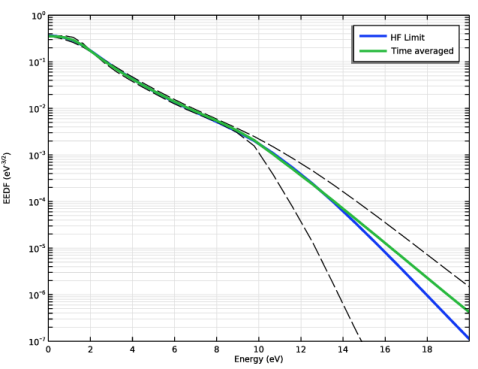
In the Settings window for 1D Plot Group, type EEDF HF Limit vs. Time Averaged in the Label text field.
3
Click to expand the Title section. From the Title type list, choose None.
Line Graph 1
1
Right-click EEDF HF Limit vs. Time Averaged and choose Line Graph.
2
In the Settings window for Line Graph, locate the Data section.
3
From the Dataset list, choose HF Limit Stationary/Solution 1 (sol1).
4
From the Parameter selection (freq) list, choose From list.
5
In the Parameter values (freq (V*m^2)) list box, select 3.5355E-20.
6
Locate the Selection section. From the Selection list, choose All domains.
7
Locate the y-Axis Data section. In the Expression text field, type be.f.
8
Locate the x-Axis Data section. From the Parameter list, choose Expression.
9
In the Expression text field, type xe_be*root.comp1.be.emax.
10
Click to expand the Legends section. Select the Show legends checkbox.
11
From the Legends list, choose Manual.
12
13
Click to expand the Coloring and Style section. From the Width list, choose 3.
EEDF HF Limit vs. Time Averaged
1
In the Model Builder window, click EEDF HF Limit vs. Time Averaged.
2
In the Settings window for 1D Plot Group, locate the Plot Settings section.
3
Select the x-axis label checkbox. In the associated text field, type Energy (eV).
4
Select the y-axis label checkbox. In the associated text field, type EEDF (eV<sup>-3/2</sup>).
5
Locate the Axis section. Select the y-axis log scale checkbox.
6
Select the Manual axis limits checkbox.
7
In the x minimum text field, type 0.
8
In the x maximum text field, type 20.
9
In the y minimum text field, type 1e-7.
10
In the y maximum text field, type 1.
11
In the EEDF HF Limit vs. Time Averaged toolbar, click  Plot.
The next step is to solve for the temporal evolution of the EEDF. Add a Time Dependent study and choose to solve the time-dependent EEDF.
Add Study
1
In the Home toolbar, click  Add Study to open the Add Study window.
2
Go to the Add Study window.
3
Find the Studies subsection. In the Select Study tree, select General Studies > Time Dependent.
4
Click the Add Study button in the window toolbar.
5
In the Home toolbar, click  Add Study to close the Add Study window.
Study 2
Step 1: Time Dependent
1
In the Settings window for Time Dependent, locate the Study Settings section.
2
In the Output times text field, type range(0,(5/f0-0)/4,5/f0) range(5/f0,(6/f0-(5/f0))/24,6/f0).
3
Click to expand the Values of Dependent Variables section. Find the Initial values of variables solved for subsection. From the Settings list, choose User controlled.
4
From the Method list, choose Solution.
5
From the Study list, choose HF Limit Stationary, Reduced Electric Fields.
6
From the Parameter value (freq (V*m^2)) list, choose From list.
7
In the Parameter value (freq (V*m^2)) list box, select 5E-20 V*m^2.
8
In the Model Builder window, click Study 2.
9
In the Settings window for Study, locate the Study Settings section.
10
Clear the Generate default plots checkbox.
Boltzmann Equation, Two-Term Approximation (be)
1
In the Model Builder window, under Component 1 (comp1) click Boltzmann Equation, Two-Term Approximation (be).
2
In the Settings window for Boltzmann Equation, Two-Term Approximation, locate the Electron Energy Distribution Function Settings section.
3
From the Temporal behavior list, choose Time dependent EEDF.
Boltzmann Model 1
1
In the Model Builder window, under Component 1 (comp1) > Boltzmann Equation, Two-Term Approximation (be) click Boltzmann Model 1.
2
In the Settings window for Boltzmann Model, locate the Boltzmann Settings section.
3
In the pA text field, type p0.
4
In the E/N text field, type EN*cos(2*pi*f0*t).
Plot the EEDFs at the instants where the tail is at its maximum and minimum values. Also, plot the time-averaged EEDF.
Time Dependent
1
In the Study toolbar, click  Compute.
2
In the Model Builder window, click Study 2.
3
In the Settings window for Study, type Time Dependent in the Label text field.
Results
Line Graph 2
1
In the Model Builder window, right-click EEDF HF Limit vs. Time Averaged and choose Line Graph.
2
In the Settings window for Line Graph, locate the Data section.
3
From the Dataset list, choose Time Dependent/Solution 2 (sol2).
4
From the Time selection list, choose From list.
5
In the Times (s) list, choose 2.0578E-9 and 2.1599E-9.
6
Locate the Selection section. From the Selection list, choose All domains.
7
Locate the y-Axis Data section. In the Expression text field, type be.f.
8
Locate the x-Axis Data section. From the Parameter list, choose Expression.
9
In the Expression text field, type xe_be*root.comp1.be.emax.
10
Locate the Coloring and Style section. Find the Line style subsection. From the Line list, choose Dashed.
11
From the Color list, choose Black.
12
In the EEDF HF Limit vs. Time Averaged toolbar, click  Plot.
Line Graph 3
1
Right-click EEDF HF Limit vs. Time Averaged and choose Line Graph.
2
In the Settings window for Line Graph, locate the Data section.
3
From the Dataset list, choose Time Dependent/Solution 2 (sol2).
4
From the Time selection list, choose Last.
5
Locate the Selection section. From the Selection list, choose All domains.
6
Locate the y-Axis Data section. In the Expression text field, type timeavg(5/f0, 6/f0, be.f).
7
Locate the x-Axis Data section. From the Parameter list, choose Expression.
8
In the Expression text field, type xe_be*root.comp1.be.emax.
9
Locate the Coloring and Style section. From the Width list, choose 3.
10
Locate the Legends section. Select the Show legends checkbox.
11
From the Legends list, choose Manual.
12
13
In the EEDF HF Limit vs. Time Averaged toolbar, click  Plot.
Add one last study to parameterize over the reduced field and obtain transport parameters and rate coefficients as functions of the electron mean energy.
Boltzmann Equation, Two-Term Approximation (be)
1
In the Model Builder window, under Component 1 (comp1) click Boltzmann Equation, Two-Term Approximation (be).
2
In the Settings window for Boltzmann Equation, Two-Term Approximation, locate the Electron Energy Distribution Function Settings section.
3
From the Temporal behavior list, choose Stationary EEDF.
Add Study
1
In the Home toolbar, click  Add Study to open the Add Study window.
2
Go to the Add Study window.
3
Find the Studies subsection. In the Select Study tree, select Preset Studies for Selected Physics Interfaces > Reduced Electric Fields.
4
Click the Add Study button in the window toolbar.
5
In the Home toolbar, click  Add Study to close the Add Study window.
Study 3
Step 1: Reduced Electric Fields
1
In the Settings window for Reduced Electric Fields, locate the Study Settings section.
2
In the Reduced electric fields text field, type range(10,10,500)[Td].
3
In the Model Builder window, click Study 3.
4
In the Settings window for Study, locate the Study Settings section.
5
Clear the Generate default plots checkbox.
6
In the Label text field, type HF Limit parameterization.
7
In the Study toolbar, click  Compute.
Results
EEDFs
1
In the Results toolbar, click  1D Plot Group.
2
In the Settings window for 1D Plot Group, type EEDFs in the Label text field.
3
Locate the Data section. From the Dataset list, choose HF Limit parameterization/Solution 3 (sol3).
Line Graph 1
1
Right-click EEDFs and choose Line Graph.
2
In the Settings window for Line Graph, locate the Selection section.
3
From the Selection list, choose All domains.
4
Locate the y-Axis Data section. In the Expression text field, type be.f.
5
Locate the x-Axis Data section. From the Parameter list, choose Expression.
6
In the Expression text field, type xe_be*root.comp1.be.emax.
EEDFs
1
In the Model Builder window, click EEDFs.
2
In the Settings window for 1D Plot Group, locate the Title section.
3
From the Title type list, choose None.
4
Locate the Plot Settings section.
5
Select the x-axis label checkbox. In the associated text field, type Energy (eV).
6
Select the y-axis label checkbox. In the associated text field, type EEDF (eV<sup>-3/2</sup>).
7
Locate the Axis section. Select the y-axis log scale checkbox.
8
Select the Manual axis limits checkbox.
9
In the x minimum text field, type 0.
10
In the x maximum text field, type 200.
11
In the y minimum text field, type 1e-7.
12
In the y maximum text field, type 2.
13
Locate the Legend section. Clear the Show legends checkbox.
14
In the EEDFs toolbar, click  Plot.
Electron Mean Energy vs. E/N
1
In the Results toolbar, click  1D Plot Group.
2
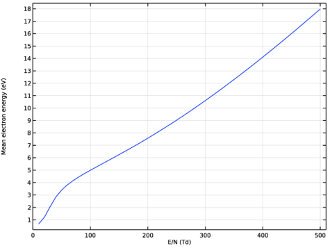
In the Settings window for 1D Plot Group, type Electron Mean Energy vs. E/N in the Label text field.
3
Locate the Data section. From the Dataset list, choose HF Limit parameterization/Solution 3 (sol3).
Global 1
1
Right-click Electron Mean Energy vs. E/N and choose Global.
2
In the Settings window for Global, locate the y-Axis Data section.
3
4
Locate the x-Axis Data section. From the Unit list, choose Td.
Electron Mean Energy vs. E/N
1
In the Model Builder window, click Electron Mean Energy vs. E/N.
2
In the Settings window for 1D Plot Group, locate the Title section.
3
From the Title type list, choose None.
4
Locate the Plot Settings section.
5
Select the x-axis label checkbox. In the associated text field, type E/N (Td).
6
Select the y-axis label checkbox. In the associated text field, type Mean electron energy (eV).
7
In the Electron Mean Energy vs. E/N toolbar, click  Plot.
8
Locate the Legend section. Clear the Show legends checkbox.
Electron Mobility vs. Electron Mean Energy
1
In the Results toolbar, click  1D Plot Group.
2
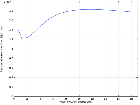
In the Settings window for 1D Plot Group, type Electron Mobility vs. Electron Mean Energy in the Label text field.
3
Locate the Data section. From the Dataset list, choose HF Limit parameterization/Solution 3 (sol3).
4
Locate the Title section. From the Title type list, choose None.
Global 1
1
Right-click Electron Mobility vs. Electron Mean Energy and choose Global.
2
In the Settings window for Global, locate the y-Axis Data section.
3
4
Locate the x-Axis Data section. From the Parameter list, choose Expression.
5
In the Expression text field, type be.ebar.
Electron Mobility vs. Electron Mean Energy
1
In the Model Builder window, click Electron Mobility vs. Electron Mean Energy.
2
In the Settings window for 1D Plot Group, locate the Plot Settings section.
3
Select the x-axis label checkbox. In the associated text field, type Mean electron energy (eV).
4
Locate the Axis section. Select the Manual axis limits checkbox.
5
In the x minimum text field, type 0.
6
In the x maximum text field, type 19.
7
In the y minimum text field, type 0.
8
In the y maximum text field, type 2e24.
9
Locate the Legend section. Clear the Show legends checkbox.
10
In the Electron Mobility vs. Electron Mean Energy toolbar, click  Plot.
Ionization Rate Constants vs. Electron Mean Energy
1
In the Results toolbar, click  1D Plot Group.
2
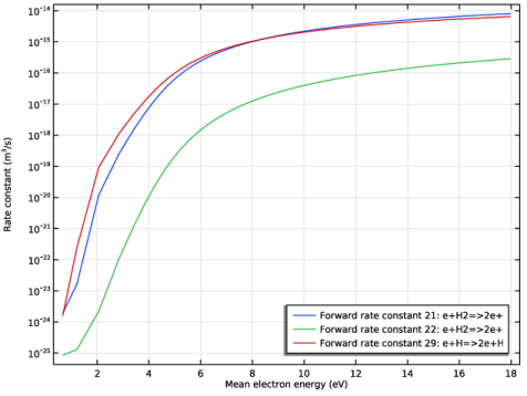
In the Settings window for 1D Plot Group, type Ionization Rate Constants vs. Electron Mean Energy in the Label text field.
3
Locate the Data section. From the Dataset list, choose HF Limit parameterization/Solution 3 (sol3).
4
Locate the Title section. From the Title type list, choose None.
Global 1
1
Right-click Ionization Rate Constants vs. Electron Mean Energy and choose Global.
2
In the Settings window for Global, locate the y-Axis Data section.
3
4
Locate the x-Axis Data section. From the Parameter list, choose Expression.
5
In the Expression text field, type be.ebar.
6
Click to expand the Legends section. In the Ionization Rate Constants vs. Electron Mean Energy toolbar, click  Plot.
Ionization Rate Constants vs. Electron Mean Energy
1
In the Model Builder window, click Ionization Rate Constants vs. Electron Mean Energy.
2
In the Settings window for 1D Plot Group, locate the Plot Settings section.
3
Select the x-axis label checkbox. In the associated text field, type Mean electron energy (eV).
4
Select the y-axis label checkbox. In the associated text field, type Rate constant (m<sup>3</sup>/s).
5
Locate the Axis section. Select the y-axis log scale checkbox.
6
Locate the Legend section. From the Position list, choose Lower right.