COMSOL 6.4 - Insulation of a Pipeline Section

As oil flows through a pipeline, heat is dissipated due to internal viscous shear in the fluid. With good insulation of the pipeline, this generated heat can be used to avoid the need of preheating of the oil, despite the fact that it needs to be transported in a cold environment over long distances.

This model uses the Nonisothermal Pipe Flow interface to set up and solve the flow and energy equations describing oil transport in a pipeline section. With the addition of an Optimization study, the thickness of the pipeline insulation can be found such that the temperature is constant along the pipe stretch.

The third study in this application requires the Optimization Module.

Model Definition

Oil flowing at a rate of 2500 m3/h enters a 150 km pipeline section with a temperature of 25°C. The average temperature outside of the pipeline is −10°C.

Figure 1: A section of pipeline transporting crude oil.

Flow Equations

The continuity and momentum equations below describe the flow of oil inside a horizontal pipe:

(1)

Above, A (SI unit: m2) is the cross section area of the pipe, ρ (SI unit: kg/m3) is the density, u (SI unit: m/s) is the fluid velocity, and p (SI unit: N/m2) is the pressure.

The second term on the right-hand side of Equation 1 describes the pressure drop due to internal viscous shear. The term contains the Darcy friction factor, fD, which is a function of the Reynolds number and the surface roughness divided by the hydraulic pipe diameter. In this example, fD is calculated from the Haaland equation (Ref. 1). It can recover both small and large relative roughness limits for a wide range of Reynolds numbers (4·103 < Re < 1·108):

(2)

The pipe flow interfaces have the Haaland equation and several other friction models predefined and automatically calculate the friction factor based on the local properties of the pipe, the fluid physical properties, and the fluid velocity.

Heat Transfer Equations

The energy equation the pipeline flow is:

(3)

where Cp (SI unit: J/(kg·K)) is the heat capacity at constant pressure, T is the temperature (SI unit: K), and k (SI unit: W/(m·K)) is the thermal conductivity. The second term on the right-hand side of Equation 3 corresponds to heat released due to the work of internal friction forces. Qwall (SI unit: W/m) is a source/sink term due to heat exchange with the surroundings through the pipe wall:

Where Z (m) is the perimeter of the pipe, h (W/(m2·K)) an overall heat transfer coefficient and Text (K) the external temperature outside the pipe.

The overall heat transfer coefficient includes contribution from internal film resistance, wall resistance, and external film resistance.

For a circular pipe, assuming equal temperature around the circumference of the pipe, and that the heat transfer through the wall is quasi static, an effective hZ in Equation 3 is given by

where rn is the outer radius of wall n, hint, and hext are the film heat transfer coefficients on the inside and outside of the tube, respectively, and kn is the thermal conductivity of wall n. In this model, the pipe wall and one layer of insulation is modeled (Figure 2)

Figure 2: Pipeline cross section. A two layered wall (dark and light gray) and the film resistances on the inside and outside (light blue).

Properties of the pipe and insulation material is given in the table below.

Table 1: Pipe properties.
name	value	description
dwall	2 cm	Pipe wall thickness
kwall	45 W/(m·K)	Pipe wall thermal conductivity
dins	To be determined	Insulation thickness
kins	0.025 W/(m·K)	Insulation thermal conductivity

The film resistance inside the pipe is given by:

with the following Nusselt correlation (Ref. 2):

The film resistance due to the external flow of air around the pipeline is:

where Nuext is calculated with a forced convection relation, assuming an average air speed of 5 m/s.

Results and Discussion

A first study calculates the temperature along the pipeline assuming perfect insulation, as well as case where the pipeline in uninsulated. Figure 3 shows that the heat generated due to friction increases the temperature of the oil by approximately 3°C over 150 km. With no pipeline insulation the temperature at the outlet is close to that of the surroundings.

Figure 3: Oil temperature as a function of position in the pipeline assuming no heat transfer across the pipe wall, heat transfer with no insulating material around the pipe, and with an optimized insulation thickness.

Optimization calculations performed under the constraint that the temperature at the outlet should be the same as inlet temperature, predicts that the thickness of the insulating material should be approximately 8.6 cm.

It is always advisable to check the Reynolds number and verify that the friction model is valid under the present flow conditions. In this case Re = 1.1·105 confirming that the Haaland equation is valid for calculating fD.

Figure 4shows the temperature distribution in the pipe insulation layer visualized using a special Pipe dataset.

Figure 4: Temperature distribution.

Notes About the COMSOL Implementation

This modeling example involves three study.

The oil’s temperature is calculated accounting for friction heating and heat lost to the surroundings when the pipeline is uninsulated.

The other extreme case is computed: perfect insulation (no heat leakage to the surroundings).

The optimal thickness of an insulating layer is computed through optimization. The insulation thickness is sought so that the outlet temperature is equal to the inlet temperature.

References

1. S.E. Haaland, “Simple and Explicit Formulas for the Friction Factor in Turbulent Flow,” J. Fluids Engineering (ASME), vol. 103, no. 5, pp. 89–90, 1983.

2. F.P. Incropera and D.P. DeWitt, Fundamentals of Heat and Mass Transfer, 4th ed., John Wiley & Sons, 1996. Eq 8.62 and Eq 7.55, respectively.

Pipe_Flow_Module/Heat_Transfer/pipeline_insulation

Modeling Instructions

From the menu, choose .

New

In the window, click

Model Wizard

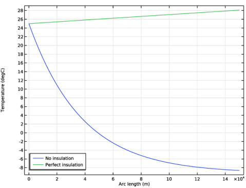
In the window, Start by setting up the nonisothermal flow problem, solving for the cases of perfect insulation and no insulation of the pipeline.

click

In the tree, select > > .

Click .

Click

In the tree, select > .

Click

Geometry 1

Polygon 1 (pol1)

In the toolbar, click

and choose .

In the window for , locate the section.

In the table, enter the following settings:


x (m)	y (m)	z (m)
0	0	0
0	0	0
150e3	0	0

Click

Next, import parameter values from text file.

Global Definitions

Parameters 1

In the window, under click .

In the window for , locate the section.

Click

Browse to the model’s Application Libraries folder and double-click the file pipeline_insulation_parameters.txt.

Materials

Now create the crude oil material needed for the simulation. The air properties needed for the external forced convection cooling is taken from the built-in materials database.

Crude oil

In the window, under right-click and choose .

In the window for , type Crude oil in the text field.

Locate the section. In the table, enter the following settings:


Property	Variable	Value	Unit	Property group
Density	rho	rho_oil	kg/m³	Basic
Dynamic viscosity	mu	mu_oil	Pa·s	Basic
Heat capacity at constant pressure	Cp	Cp_oil	J/(kg·K)	Basic
Ratio of specific heats	gamma	gamma_oil	1	Basic
Thermal conductivity	k_iso ; kii = k_iso, kij = 0	k_oil	W/(m·K)	Basic