PDF

Topology Optimization of a District Heating Network
Introduction
Power plants utilizing cogeneration can reach high efficiencies in winter time, but they rely on district heating networks. The design of such networks has previously been limited to inaccurate linear models or nonlinear models of small networks. Recent research has demonstrated gradient-based optimization for designing large networks using nonlinear models (Ref. 2). This model reproduces this research using the Pipe Flow Module and Optimization Module of COMSOL Multiphysics. Power plants for electricity generation often convert less than half the input energy to electrical energy. It is possible to increase the efficiency by capturing the heat generated in the process. The heat can be used for residential heating in urban environments, but to realize this one has to construct a network of pipes for distributing the heat. The technology can allow efficiencies up to 80% in winter time Ref. 1.
Model Definition
The model considers identical consumers, continuous pipe diameters, and a simple models for the radiators and network heat loss. This means that the resulting network topology is likely to be good, but to be able to trust the quantitative values for the pipe diameters it might be necessary to use more advanced expressions and techniques as has been done in Ref. 2.
Figure 1: The initial geometry.
The initial geometry for this model is shown in Figure 1.
The optimization problem consists of controls, constraints, and objectives.
Controls
District heating network are generally aligned with the road infrastructure, so the question of how the network should be designed can be reduced to a question of which roads should have pipes and how large should the pipes be. The consumers are generally (financially) punished for returning the heated water too hot, because this constitutes a waste of pumping energy. Consumers thus have an incentive to decrease the flow speed over the heat exchanger that connects the heating network to their heating system of their property. This can lead low flow rates in the system, which can cause low temperatures for consumers far from the producer due to heat lost from the network to the earth. To prevent this issue, the heating network is equipped with bypass valves in the end of the network so that an adequate flow rate can be ensured. Because the endpoints of the network are not known, treat each producer as a bypass valve and optimize the diameter of this. Also, optimize the coupling constant to the network, which corresponds to a setting for the consumer heating system. Finally, allow the driving pressure over the network to be optimized.
Constraints
In order for the network to be valid it has to be able to distribute sufficient heat to all consumers, but a large network will have many consumers leading to many constraints, which can be numerically problematic. A popular solution to this problem is to use a constraint aggregation technique, so that a large number of linear constraints is converted to a single nonlinear constraint, that is
The violation of local constraints will decrease with larger values of β, but the large values will also cause numerical problems, so in practice a compromise has to be found.
Objective
The primary cost of establishing the network is related to the total length of trenches that have to be dug, but larger pipes also cost more than smaller pipes, so the cost can be approximated as
where D is the pipe diameter and b is the cost of digging a trench. By itself, this would lead to a network with very small pipes and a large pressure drop requiring an expensive pump. This can be avoided by adding a term related to the pumping power, so that the total objective function becomes
The constant relating the pumping power to the objective function depends on several factors, such as the maintenance cost of the network, the price of electricity, and the cost of capital.
Results and Discussion
Figure 2: The network topology is shown with the consumer heating powers. The minimum power is 4.7 kW, so none of the consumers are freezing.
Each consumers requires 5 kW of heating power. Two heat producers with in flow temperatures of 65 and 70°C are considered (top and lower right, respectively). The model starts out by optimizing the bypass and radiator controls, with the constraint, C, as the objective function. The result of this is used as initial guess, when minimizing EURtotal.
Figure 2 shows the optimized pipe diameters together with the heating power for each consumer. The network design branches into smaller and smaller pipes as one would expect. In this case, consider a situation, where there are consumers almost everywhere, and this makes it difficult to reduce EURpipes.
Figure 3: The bypass controls are primarily open in the end of the network far from the producers.
Figure 3 shows the values of the bypass controls. As expected larger values appear in the very end of the network. Finally, Figure 4 illustrates that the consumers belonging to the network with a 65°C inlet temperature need slightly better radiators, particularly far from the producer.
Figure 4: The consumer radiator controls are slightly larger in the network belonging to the upper producer.
References
1. www.energy.gov/fecm/how-gas-turbine-power-plants-work
2. M. Blommaert, Y. Wack, and M. Baelmans, “An adjoint optimization approach for the topological design of large-scale district heating networks based on nonlinear models,” Applied Energy, vol. 280, p. 116025, 2020.
Notes About the COMSOL Implementation
The original MMA optimization solver (which is not globally convergent) is used to avoid premature convergence. A PDE with a Helmholtz filter is used to average the power over each consumer.
Application Library path: Pipe_Flow_Module/Heat_Transfer/district_heating_optimization
Modeling Instructions
From the File menu, choose New.
New
In the New window, click  Model Wizard.
Model Wizard
1
In the Model Wizard window, click  3D.
2
In the Select Physics tree, select Fluid Flow > Nonisothermal Flow > Nonisothermal Pipe Flow (nipfl).
3
Click Add.
4
In the Select Physics tree, select Mathematics > PDE Interfaces > Lower Dimensions > Coefficient Form Edge PDE (ce).
5
Click Add.
6
In the Field name (1) text field, type P.
7
In the Dependent variables (1) table, enter the following settings:
8
Click  Select Dependent Variable Quantity.
9
In the Physical Quantity dialog, type power in the text field.
10
In the tree, select General > Power (W).
11
12
In the Model Wizard window, click  Select Source Term Quantity.
13
In the Physical Quantity dialog, type power in the text field.
14
In the tree, select General > Power (W).
15
16
In the Model Wizard window, click  Study.
17
In the Select Study tree, select General Studies > Stationary.
18
Geometry 1
Create the geometry. To simplify this step, insert a prepared geometry sequence.
1
In the Geometry toolbar, click Insert Sequence and choose Insert Sequence.
2
3
In the Geometry toolbar, click  Build All.
4
Click the  Zoom Extents button in the Graphics toolbar.
5
In the Model Builder window, under Component 1 (comp1) click Geometry 1.
The geometry should now look like that in Figure 1. Note that the inserted geometry is parameterized and that the parameters used are automatically added to the list of global parameters in the model.
6
In the Model Builder window, collapse the Geometry 1 node.
Global Definitions
Geometrical Parameters
1
In the Model Builder window, under Global Definitions click Parameters 1.
2
In the Settings window for Parameters, type Geometrical Parameters in the Label text field.
Model Parameters
1
In the Home toolbar, click  Parameters and choose Add > Parameters.
2
In the Settings window for Parameters, type Model Parameters in the Label text field.
3
Locate the Parameters section. Click  Load from File.
4
Add Material
1
In the Materials toolbar, click  Add Material to open the Add Material window.
2
Go to the Add Material window.
3
In the tree, select Built-in > Water, liquid.
4
Click the Add to Component button in the window toolbar.
5
In the Materials toolbar, click  Add Material to close the Add Material window.
Definitions
Pipes
1
In the Definitions toolbar, click  Control Variables and choose Control Variable Field.
2
In the Settings window for Control Variable Field, type Pipes in the Label text field.
3
In the Name text field, type pipeControl.
4
Locate the Geometric Entity Selection section. From the Geometric entity level list, choose Edge.
5
From the Selection list, choose Hot Flow.
6
Locate the Discretization section. From the Shape function type list, choose Discontinuous Lagrange.
7
From the Element order list, choose Constant.
8
Locate the Bounds section. Select the Use bounds checkbox.
9
In the Lower bound text field, type log(0.01).
10
In the Upper bound text field, type log(2).
Bypass
1
In the Definitions toolbar, click  Control Variables and choose Control Variable Field.
2
In the Settings window for Control Variable Field, type Bypass in the Label text field.
3
In the Name text field, type bypass.
4
Locate the Geometric Entity Selection section. From the Geometric entity level list, choose Point.
5
From the Selection list, choose Consumer Hot Points.
6
Locate the Discretization section. From the Shape function type list, choose Discontinuous Lagrange.
7
From the Element order list, choose Constant.
8
Locate the Bounds section. Select the Use bounds checkbox.
9
In the Lower bound text field, type log(0.01).
10
In the Upper bound text field, type log(10).
Consumers
1
Right-click Bypass and choose Duplicate.
2
In the Settings window for Control Variable Field, type Consumers in the Label text field.
3
In the Name text field, type consumers.
4
Locate the Bounds section. In the Lower bound text field, type log(0.1).
All Pipes
1
In the Definitions toolbar, click  Nonlocal Couplings and choose Integration.
2
In the Settings window for Integration, type All Pipes in the Label text field.
3
In the Operator name text field, type intopAll.
4
Locate the Source Selection section. From the Geometric entity level list, choose Edge.
5
From the Selection list, choose All edges.
Hot Pipes
1
Right-click All Pipes and choose Duplicate.
2
In the Settings window for Integration, type Hot Pipes in the Label text field.
3
In the Operator name text field, type intopHot.
4
Locate the Source Selection section. From the Selection list, choose Hot Flow.
Consumers
1
Right-click Hot Pipes and choose Duplicate.
2
In the Settings window for Integration, type Consumers in the Label text field.
3
In the Operator name text field, type intopConsumers.
4
Locate the Source Selection section. From the Selection list, choose Consumers.
Inlet 1
1
Right-click Consumers and choose Duplicate.
2
In the Settings window for Integration, type Inlet 1 in the Label text field.
3
In the Operator name text field, type intopInlet1.
4
Locate the Source Selection section. From the Geometric entity level list, choose Point.
5
From the Selection list, choose Inlet 1.
Outlet 1
1
Right-click Inlet 1 and choose Duplicate.
2
In the Settings window for Integration, type Outlet 1 in the Label text field.
3
In the Operator name text field, type intopOutlet1.
4
Locate the Source Selection section. From the Selection list, choose Outlet 1.
Outlet 2
1
Right-click Outlet 1 and choose Duplicate.
2
In the Settings window for Integration, type Outlet 2 in the Label text field.
3
Locate the Source Selection section. From the Selection list, choose Outlet 2.
Inlet 2
1
Right-click Outlet 2 and choose Duplicate.
2
In the Settings window for Integration, type Inlet 2 in the Label text field.
3
In the Operator name text field, type intopInlet2.
4
Locate the Source Selection section. From the Selection list, choose Inlet 2.
Consumer Average
1
In the Definitions toolbar, click  Nonlocal Couplings and choose Average.
2
In the Settings window for Average, type Consumer Average in the Label text field.
3
In the Operator name text field, type aveopConsumer.
4
Locate the Source Selection section. From the Geometric entity level list, choose Edge.
5
From the Selection list, choose Consumers.
Consumer Minimum
1
In the Definitions toolbar, click  Nonlocal Couplings and choose Minimum.
2
In the Settings window for Minimum, type Consumer Minimum in the Label text field.
3
Locate the Source Selection section. From the Geometric entity level list, choose Point.
4
From the Selection list, choose Consumer Hot Points.
General Extrusion 1 (genext1)
1
In the Definitions toolbar, click  Nonlocal Couplings and choose General Extrusion.
2
In the Settings window for General Extrusion, locate the Source Selection section.
3
From the Geometric entity level list, choose Edge.
4
From the Selection list, choose Hot Flow.
5
Locate the Destination Map section. In the z-expression text field, type 0.
General Extrusion 2 (genext2)
1
Right-click General Extrusion 1 (genext1) and choose Duplicate.
2
In the Settings window for General Extrusion, locate the Source Selection section.
3
From the Geometric entity level list, choose Point.
4
From the Selection list, choose Consumer Hot Points.
In the Model Builder Window, under Component 1 (comp1) > Definitions, Ctrl-click to select all nonlocal coupling operators. Then right-click and choose Group.
Operators
1
In the Model Builder window, under Component 1 (comp1) > Definitions click Group 1.
2
In the Settings window for Group, type Operators in the Label text field.
Pipe Cost
1
In the Definitions toolbar, click  Analytic.
2
In the Settings window for Analytic, type Pipe Cost in the Label text field.
3
In the Function name text field, type pipeCost.
4
Locate the Definition section. In the Expression text field, type 2202+(2922-2202)*(x-0.032)/(0.4-0.032).
The values are taken from Ref. 2.
5
Locate the Units section. In the Function text field, type 1/m.
6
Hot Pipes
1
In the Model Builder window, right-click Definitions and choose Variables.
2
In the Settings window for Variables, type Hot Pipes in the Label text field.
3
Locate the Geometric Entity Selection section. From the Geometric entity level list, choose Edge.
4
From the Selection list, choose Hot Flow.
5
Locate the Variables section. In the table, enter the following settings:
Cold Pipes
1
Right-click Hot Pipes and choose Duplicate.
2
In the Settings window for Variables, type Cold Pipes in the Label text field.
3
Locate the Geometric Entity Selection section. From the Selection list, choose Cold Flow.
4
Locate the Variables section. In the table, enter the following settings:
This enforces identical pipe diameters for hot and cold flows.
Consumers
1
Right-click Cold Pipes and choose Duplicate.
2
In the Settings window for Variables, type Consumers in the Label text field.
3
Locate the Geometric Entity Selection section. From the Selection list, choose Consumers.
4
Locate the Variables section. In the table, enter the following settings:
Inlet/Outlet
1
Right-click Consumers and choose Duplicate.
2
In the Settings window for Variables, type Inlet/Outlet in the Label text field.
3
Locate the Geometric Entity Selection section. From the Selection list, choose Inlets+Outlets.
4
Locate the Variables section. In the table, enter the following settings:
Objectives
1
In the Model Builder window, right-click Definitions and choose Variables.
2
In the Settings window for Variables, type Objectives in the Label text field.
You can import the table contents from district_heating_optimization_variables.txt.
3
Locate the Variables section. In the table, enter the following settings:
Nonisothermal Pipe Flow (nipfl)
Pipe Properties 1
1
In the Model Builder window, under Component 1 (comp1) > Nonisothermal Pipe Flow (nipfl) click Pipe Properties 1.
2
In the Settings window for Pipe Properties, locate the Pipe Shape section.
3
4
In the di text field, type pipeD.
Pressure 1
1
In the Model Builder window, click Pressure 1.
2
In the Settings window for Pressure, locate the Boundary Pressure section.
3
In the p0 text field, type 1[atm].
Temperature 1
1
In the Model Builder window, click Temperature 1.
2
In the Settings window for Temperature, locate the Temperature section.
3
In the Tin text field, type T1.
Heat Source 1
1
In the Physics toolbar, click  Edges and choose Heat Source.
2
In the Settings window for Heat Source, locate the Edge Selection section.
3
From the Selection list, choose All edges.
4
Locate the Heat Source section. In the Q0 text field, type qHeat.
Pressure 2
1
In the Physics toolbar, click  Points and choose Pressure.
2
In the Settings window for Pressure, locate the Point Selection section.
3
From the Selection list, choose Inlet 1.
4
Locate the Boundary Pressure section. In the p0 text field, type 1[atm]+dp1*exp(dp1c).
Pressure 3
1
Right-click Pressure 2 and choose Duplicate.
2
In the Settings window for Pressure, locate the Point Selection section.
3
From the Selection list, choose Inlet 2.
4
Locate the Boundary Pressure section. In the p0 text field, type 1[atm]+dp2*exp(dp2c).
Temperature 2
1
In the Physics toolbar, click  Points and choose Temperature.
2
In the Settings window for Temperature, locate the Point Selection section.
3
From the Selection list, choose Inlet 2.
4
Locate the Temperature section. In the Tin text field, type T2.
Heat Outflow 1
1
In the Physics toolbar, click  Points and choose Heat Outflow.
2
In the Settings window for Heat Outflow, locate the Point Selection section.
3
From the Selection list, choose Outlet 1.
Heat Outflow 2
1
Right-click Heat Outflow 1 and choose Duplicate.
2
In the Settings window for Heat Outflow, locate the Point Selection section.
3
From the Selection list, choose Outlet 2.
Average Consumer Power
1
In the Model Builder window, under Component 1 (comp1) click Coefficient Form Edge PDE (ce).
2
In the Settings window for Coefficient Form Edge PDE, type Average Consumer Power in the Label text field.
3
Locate the Edge Selection section. From the Selection list, choose Consumers.
Coefficient Form PDE 1
1
In the Model Builder window, under Component 1 (comp1) > Average Consumer Power (ce) click Coefficient Form PDE 1.
2
In the Settings window for Coefficient Form PDE, locate the Diffusion Coefficient section.
3
In the c text field, type 1e6*Lz^2.
4
Locate the Absorption Coefficient section. In the a text field, type 1.
5
Locate the Source Term section. In the f text field, type qHeat*Lz.
This effectively averages the power over each consumer.
Mesh 1
1
In the Model Builder window, under Component 1 (comp1) click Mesh 1.
2
In the Settings window for Mesh, locate the Physics-Controlled Mesh section.
3
From the Element size list, choose Extremely fine.
Study 1: Initial Design
1
In the Model Builder window, click Study 1.
2
In the Settings window for Study, type Study 1: Initial Design in the Label text field.
3
In the Study toolbar, click  Get Initial Value.
Solver Configurations
In the Model Builder window, expand the Study 1: Initial Design > Solver Configurations node.
Solution 1 (sol1)
Use a Segregated solver to improve robustness.
1
In the Model Builder window, expand the Study 1: Initial Design > Solver Configurations > Solution 1 (sol1) node.
2
Right-click Stationary Solver 1 and choose Segregated.
3
Right-click Segregated 1 and choose Segregated Step.
4
In the Settings window for Segregated Step, type Temperature in the Label text field.
5
Locate the General section. Under Variables, click  Add.
6
In the Add dialog, in the Variables list, choose Control Variable Field (comp1.bypass), Control Variable Field (comp1.consumers), Control Variable Field (comp1.pipeControl), and Temperature (comp1.T).
7
8
Right-click Segregated 1 and choose Segregated Step.
9
In the Settings window for Segregated Step, type Power in the Label text field.
10
Locate the General section. Under Variables, click  Add.
11
In the Add dialog, in the Variables list, choose Control Variable Field (comp1.bypass), Control Variable Field (comp1.consumers), Dependent Variable P (comp1.P), and Control Variable Field (comp1.pipeControl).
12
13
In the Model Builder window, under Study 1: Initial Design > Solver Configurations > Solution 1 (sol1) > Stationary Solver 1 > Segregated 1 click Segregated Step.
14
In the Settings window for Segregated Step, type Flow in the Label text field.
15
Locate the General section. In the Variables list, choose Dependent Variable P (comp1.P) and Temperature (comp1.T).
16
Under Variables, click  Delete.
17
In the Study toolbar, click  Compute.
Results
Average Consumer Power
In the Model Builder window, under Results right-click Average Consumer Power and choose Delete.
Arrow Line 1
1
In the Model Builder window, expand the Results > Velocity (nipfl) node, then click Arrow Line 1.
2
In the Settings window for Arrow Line, locate the Arrow Positioning section.
3
From the Placement list, choose Gauss points.
4
In the Velocity (nipfl) toolbar, click  Plot.
Line 1
1
In the Model Builder window, expand the Results > Temperature (nipfl) node, then click Line 1.
2
In the Settings window for Line, locate the Expression section.
3
In the Unit field, type degC.
4
In the Temperature (nipfl) toolbar, click  Plot.
Pressure (nipfl), Temperature (nipfl), Velocity (nipfl)
1
In the Model Builder window, under Results, Ctrl-click to select Pressure (nipfl), Velocity (nipfl), and Temperature (nipfl).
2
Initial Design
In the Settings window for Group, type Initial Design in the Label text field.
Add Study
1
In the Home toolbar, click  Add Study to open the Add Study window.
2
Go to the Add Study window.
3
Find the Studies subsection. In the Select Study tree, select General Studies > Stationary.
4
Click the Add Study button in the window toolbar.
5
Click the Add Study button in the window toolbar.
6
In the Home toolbar, click  Add Study to close the Add Study window.
Study 2
General Optimization
1
In the Study toolbar, click  Optimization and choose General Optimization.
2
In the Settings window for General Optimization, locate the Optimization Solver section.
3
From the Method list, choose GCMMA.
4
In the Maximum number of model evaluations text field, type 50.
The controls are logarithmic, so enabling move limits prevents MMA from making relative adjustments larger than exp(0.1). This improves robustness of the optimization.
Start out by varying the bypass and consumer controls, so that the constraint is minimized.
5
Click Add Expression in the upper-right corner of the Objective Function section. From the menu, choose Component 1 (comp1) > Definitions > Variables > comp1.constr - Constraint.
6
Locate the Objective Function section. In the table, enter the following settings:
7
In the Model Builder window, click Study 2.
8
In the Settings window for Study, locate the Study Settings section.
9
Clear the Generate default plots checkbox.
10
In the Label text field, type Study 2: Feasible Design.
11
In the Study toolbar, click  Get Initial Value.
Solver Configurations
In the Model Builder window, expand the Study 2: Feasible Design > Solver Configurations node.
Solution 2 (sol2)
1
In the Model Builder window, expand the Study 2: Feasible Design > Solver Configurations > Solution 2 (sol2) node, then click Optimization Solver 1.
2
In the Settings window for Optimization Solver, locate the Optimization Solver section.
3
Select the Move limits checkbox.
4
In the Model Builder window, expand the Study 2: Feasible Design > Solver Configurations > Solution 2 (sol2) > Optimization Solver 1 node.
5
Right-click Stationary Solver 1 and choose Segregated.
6
In the Model Builder window, expand the Study 2: Feasible Design > Solver Configurations > Solution 2 (sol2) > Optimization Solver 1 > Stationary Solver 1 > Segregated 1 node.
7
Right-click Segregated 1 and choose Segregated Step.
8
In the Model Builder window, collapse the Study 2: Feasible Design > Solver Configurations > Solution 2 (sol2) > Optimization Solver 1 > Stationary Solver 1 > Segregated 1 node.
9
In the Model Builder window, under Study 2: Feasible Design > Solver Configurations > Solution 2 (sol2) > Optimization Solver 1 > Stationary Solver 1 > Segregated 1 click Segregated Step 1.
10
In the Settings window for Segregated Step, type Temperature in the Label text field.
11
Locate the General section. Under Variables, click  Add.
12
In the Add dialog, in the Variables list, choose Control Variable Field (comp1.bypass), Control Variable Field (comp1.consumers), Control Variable Field (comp1.pipeControl), and Temperature (comp1.T).
13
14
In the Model Builder window, right-click Segregated 1 and choose Segregated Step.
15
In the Settings window for Segregated Step, type Power in the Label text field.
16
Locate the General section. Under Variables, click  Add.
17
In the Add dialog, in the Variables list, choose Control Variable Field (comp1.bypass), Control Variable Field (comp1.consumers), Dependent Variable P (comp1.P), and Control Variable Field (comp1.pipeControl).
18
19
In the Model Builder window, under Study 2: Feasible Design > Solver Configurations > Solution 2 (sol2) > Optimization Solver 1 > Stationary Solver 1 > Segregated 1 click Segregated Step.
20
In the Settings window for Segregated Step, type Flow in the Label text field.
21
Locate the General section. In the Variables list, choose Dependent Variable P (comp1.P) and Temperature (comp1.T).
22
Under Variables, click  Delete.
23
In the Model Builder window, click Direct 2.
24
In the Settings window for Direct, locate the General section.
25
From the Solver list, choose PARDISO.
Results
Pressure (nipfl), Temperature (nipfl), Velocity (nipfl)
1
In the Model Builder window, under Results > Initial Design, Ctrl-click to select Pressure (nipfl), Velocity (nipfl), and Temperature (nipfl).
2
Pressure (nipfl) 1, Temperature (nipfl) 1, Velocity (nipfl) 1
Right-click and choose Move Out.
Pressure (nipfl) 1
1
In the Settings window for 3D Plot Group, locate the Data section.
2
From the Dataset list, choose Study 2: Feasible Design/Solution 2 (sol2).
Velocity (nipfl) 1
1
In the Model Builder window, click Velocity (nipfl) 1.
2
In the Settings window for 3D Plot Group, locate the Data section.
3
From the Dataset list, choose Study 2: Feasible Design/Solution 2 (sol2).
Temperature (nipfl) 1
1
In the Model Builder window, click Temperature (nipfl) 1.
2
In the Settings window for 3D Plot Group, locate the Data section.
3
From the Dataset list, choose Study 2: Feasible Design/Solution 2 (sol2).
Create a plot for showing the consumer powers during the initial optimization.
Power
1
In the Results toolbar, click  3D Plot Group.
2
In the Settings window for 3D Plot Group, type Power in the Label text field.
3
Locate the Data section. From the Dataset list, choose Study 2: Feasible Design/Solution 2 (sol2).
Line 1
1
Right-click Power and choose Line.
2
In the Settings window for Line, locate the Expression section.
3
In the Expression text field, type -P.
4
Click to expand the Range section. Select the Manual color range checkbox.
5
In the Minimum text field, type 0.8*consumerPower.
6
In the Maximum text field, type 1.2*consumerPower.
7
Locate the Coloring and Style section. From the Line type list, choose Tube.
8
In the Tube radius expression text field, type 5.
9
Select the Radius scale factor checkbox.
10
From the Color table list, choose ThermalDark.
Power, Pressure (nipfl) 1, Temperature (nipfl) 1, Velocity (nipfl) 1
1
In the Model Builder window, under Results, Ctrl-click to select Pressure (nipfl) 1, Velocity (nipfl) 1, Temperature (nipfl) 1, and Power.
2
Feasible Design
In the Settings window for Group, type Feasible Design in the Label text field.
Study 2: Feasible Design
General Optimization
1
In the Model Builder window, under Study 2: Feasible Design click General Optimization.
2
In the Settings window for General Optimization, click to expand the Output section.
3
Select the Plot checkbox.
4
From the Plot group list, choose Power.
5
In the Study toolbar, click  Compute.
Results
Feasible Design
1
In the Results toolbar, click  Evaluation Group.
2
In the Settings window for Evaluation Group, type Feasible Design in the Label text field.
3
Locate the Data section. From the Dataset list, choose Study 2: Feasible Design/Solution 2 (sol2).
Global Evaluation 1
1
Right-click Feasible Design and choose Global Evaluation.
2
In the Settings window for Global Evaluation, locate the Expressions section.
3
Click  Clear Table.
4
Click Add Expression in the upper-right corner of the Expressions section. From the menu, choose Component 1 (comp1) > Definitions > Variables > Efficiency - Network efficiency - 1.
5
Click Add Expression in the upper-right corner of the Expressions section. From the menu, choose Component 1 (comp1) > Definitions > Variables > pumpPrice - Pump price [EUR] - 1.
6
Click Add Expression in the upper-right corner of the Expressions section. From the menu, choose Component 1 (comp1) > Definitions > Variables > pipePrice - Pipe price [EUR] - 1.
7
In the Feasible Design toolbar, click  Evaluate.
Study 3
General Optimization
1
In the Study toolbar, click  Optimization and choose General Optimization.
2
In the Settings window for General Optimization, locate the Optimization Solver section.
3
From the Method list, choose MMA.
4
In the Maximum number of model evaluations text field, type 2000.
5
Click Add Expression in the upper-right corner of the Objective Function section. From the menu, choose Component 1 (comp1) > Definitions > Variables > comp1.obj - Objective function - 1.
6
Locate the Control Variables and Parameters section. Click  Add twice.
7
8
Click Add Expression in the upper-right corner of the Constraints section. From the menu, choose Component 1 (comp1) > Definitions > Variables > comp1.constr - Constraint.
9
Locate the Constraints section. In the table, enter the following settings:
10
Click to expand the Solver Settings section. Find the Objective settings subsection. From the Objective scaling list, choose Initial solution based.
11
In the Model Builder window, click Study 3.
12
In the Settings window for Study, type Study 3: Optimization in the Label text field.
13
Locate the Study Settings section. Clear the Generate default plots checkbox.
14
In the Study toolbar, click  Get Initial Value.
Solver Configurations
In the Model Builder window, expand the Study 3: Optimization > Solver Configurations node.
Solution 3 (sol3)
1
In the Model Builder window, expand the Study 3: Optimization > Solver Configurations > Solution 3 (sol3) > Optimization Solver 1 node.
2
Right-click Stationary Solver 1 and choose Segregated.
3
Right-click Segregated 1 and choose Segregated Step.
4
In the Settings window for Segregated Step, type Temperature in the Label text field.
5
Locate the General section. Under Variables, click  Add.
6
In the Add dialog, in the Variables list, choose Control Variable Field (comp1.bypass), Control Variable Field (comp1.consumers), Control Variable Field (comp1.pipeControl), and Temperature (comp1.T).
7
8
Right-click Segregated 1 and choose Segregated Step.
9
In the Settings window for Segregated Step, type Power in the Label text field.
10
Locate the General section. Under Variables, click  Add.
11
In the Add dialog, in the Variables list, choose Control Variable Field (comp1.bypass), Control Variable Field (comp1.consumers), Dependent Variable P (comp1.P), and Control Variable Field (comp1.pipeControl).
12
13
In the Model Builder window, under Study 3: Optimization > Solver Configurations > Solution 3 (sol3) > Optimization Solver 1 > Stationary Solver 1 > Segregated 1 click Segregated Step.
14
In the Settings window for Segregated Step, type Flow in the Label text field.
15
Locate the General section. In the Variables list, choose Dependent Variable P (comp1.P) and Temperature (comp1.T).
16
Under Variables, click  Delete.
17
In the Model Builder window, click Direct 2.
18
In the Settings window for Direct, locate the General section.
19
From the Solver list, choose PARDISO.
Results
Power, Pressure (nipfl) 1, Temperature (nipfl) 1, Velocity (nipfl) 1
1
In the Model Builder window, under Results > Feasible Design, Ctrl-click to select Pressure (nipfl) 1, Velocity (nipfl) 1, Temperature (nipfl) 1, and Power.
2
Power 1, Pressure (nipfl) 1.1, Temperature (nipfl) 1.1, Velocity (nipfl) 1.1
Right-click and choose Move Out.
Pressure (nipfl) 2
1
In the Settings window for 3D Plot Group, type Pressure (nipfl) 2 in the Label text field.
2
Locate the Data section. From the Dataset list, choose Study 3: Optimization/Solution 3 (sol3).
Velocity (nipfl) 2
1
In the Model Builder window, under Results click Velocity (nipfl) 1.1.
2
In the Settings window for 3D Plot Group, type Velocity (nipfl) 2 in the Label text field.
3
Locate the Data section. From the Dataset list, choose Study 3: Optimization/Solution 3 (sol3).
Temperature (nipfl) 2
1
In the Model Builder window, click Temperature (nipfl) 1.1.
2
In the Settings window for 3D Plot Group, locate the Data section.
3
From the Dataset list, choose Study 3: Optimization/Solution 3 (sol3).
4
In the Label text field, type Temperature (nipfl) 2.
Power and Pipe Diameters
1
In the Model Builder window, under Results click Power 1.
2
In the Settings window for 3D Plot Group, type Power and Pipe Diameters in the Label text field.
3
Locate the Data section. From the Dataset list, choose Study 3: Optimization/Solution 3 (sol3).
4
Click to expand the Title section. From the Title type list, choose Label.
5
Locate the Plot Settings section. Clear the Plot dataset edges checkbox.
Add the pipe diameters to the plot, so that you can use the plot to visualize the network topology during the optimization.
Line 2
1
Right-click Power and Pipe Diameters and choose Line.
2
In the Settings window for Line, click Replace Expression in the upper-right corner of the Expression section. From the menu, choose Component 1 (comp1) > Nonisothermal Pipe Flow > Pipe properties > nipfl.dh - Hydraulic diameter - m.
3
Locate the Coloring and Style section. From the Line type list, choose Tube.
4
Click thebutton. From the menu, choose Component 1 (comp1) > Nonisothermal Pipe Flow > Pipe properties > nipfl.dh - Hydraulic diameter - m.
5
In the Tube radius expression text field, type nipfl.dh/2.
6
Select the Radius scale factor checkbox. In the associated text field, type 200.
7
Click to expand the Quality section. From the Evaluation settings list, choose Manual.
8
From the Smoothing list, choose None.
Selection 1
1
Right-click Line 2 and choose Selection.
The hot and cold flows have equal diameters, so you can simplify the plot by only plotting the diameters for the hot flow.
2
In the Settings window for Selection, locate the Selection section.
3
From the Selection list, choose Hot Flow.
Power and Pipe Diameters
Next, display the pressures, the consumer power range, as well as the consumer and bypass control ranges.
Annotation 1
1
In the Model Builder window, right-click Power and Pipe Diameters and choose Annotation.
2
In the Settings window for Annotation, locate the Annotation section.
3
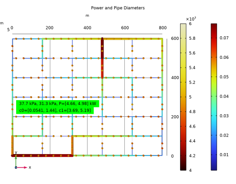
In the Text text field, type eval(dp1*exp(dp1c),kPa) kPa, eval(dp2*exp(dp2c),kPa) kPa, P=[eval(minop1(-P),kW), eval(-minop1(P),kW)] kW.
4
From the Geometry level list, choose Global.
5
Locate the Position section. In the X text field, type 20.
6
In the Y text field, type 285.
7
Click to expand the Advanced section. In the Precision text field, type 3.
8
Locate the Coloring and Style section. Clear the Show point checkbox.
9
From the Background color list, choose Green.
Annotation 2
1
Right-click Annotation 1 and choose Duplicate.
2
In the Settings window for Annotation, locate the Annotation section.
3
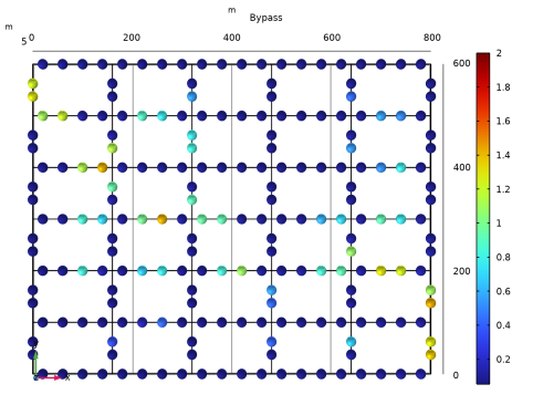
In the Text text field, type c0=[eval(minop1(exp(bypass))), eval(-minop1(-exp(bypass)))], c1=[eval(minop1(exp(consumers))), eval(-minop1(-exp(consumers)))].
4
Locate the Position section. In the Y text field, type 250.
5
Click the  Go to XY View button in the Graphics toolbar.
6
Click the  Zoom Extents button in the Graphics toolbar.
Bypass
1
In the Results toolbar, click  3D Plot Group.
2
In the Settings window for 3D Plot Group, type Bypass in the Label text field.
3
Locate the Data section. From the Dataset list, choose Study 3: Optimization/Solution 3 (sol3).
Line 1
1
Right-click Bypass and choose Line.
2
In the Settings window for Line, locate the Expression section.
3
In the Expression text field, type genext2(exp(bypass)).
4
Locate the Coloring and Style section. From the Line type list, choose Tube.
5
Select the Radius scale factor checkbox. In the associated text field, type 10.
Bypass
1
In the Model Builder window, click Bypass.
2
In the Settings window for 3D Plot Group, locate the Title section.
3
From the Title type list, choose Label.
Consumers
1
Right-click Bypass and choose Duplicate.
2
In the Model Builder window, click Bypass 1.
3
In the Settings window for 3D Plot Group, type Consumers in the Label text field.
Line 1
1
In the Model Builder window, click Line 1.
2
In the Settings window for Line, locate the Expression section.
3
In the Expression text field, type genext2(exp(consumers)).
Bypass, Consumers, Power and Pipe Diameters, Pressure (nipfl) 2, Temperature (nipfl) 2, Velocity (nipfl) 2
1
In the Model Builder window, under Results, Ctrl-click to select Pressure (nipfl) 2, Velocity (nipfl) 2, Temperature (nipfl) 2, Power and Pipe Diameters, Bypass, and Consumers.
2
Optimization
In the Settings window for Group, type Optimization in the Label text field.
Study 3: Optimization
General Optimization
1
In the Model Builder window, under Study 3: Optimization click General Optimization.
2
In the Settings window for General Optimization, locate the Output section.
3
Select the Plot checkbox.
4
From the Plot group list, choose Power and Pipe Diameters.
Step 1: Stationary
1
In the Model Builder window, click Step 1: Stationary.
2
In the Settings window for Stationary, click to expand the Values of Dependent Variables section.
3
Find the Initial values of variables solved for subsection. From the Settings list, choose User controlled.
4
From the Method list, choose Solution.
5
From the Study list, choose Study 2: Feasible Design, Stationary.
Solution 3 (sol3)
1
In the Model Builder window, under Study 3: Optimization > Solver Configurations > Solution 3 (sol3) click Optimization Solver 1.
2
In the Settings window for Optimization Solver, locate the Optimization Solver section.
3
Select the Move limits checkbox.
4
In the Study toolbar, click  Compute.
Results
Optimization
1
In the Model Builder window, right-click Feasible Design and choose Duplicate.
2
In the Settings window for Evaluation Group, type Optimization in the Label text field.
3
Locate the Data section. From the Dataset list, choose Study 3: Optimization/Solution 3 (sol3).
4
In the Optimization toolbar, click  Evaluate.
It is not possible to reduce the total pipe price too much, because there are consumers everywhere and the price is more related to the digging than the actual price of the pipes. It is however possible to reduce the pumping price significantly as well as the network efficiency.
Line 1
1
In the Model Builder window, expand the Results > Optimization > Bypass node, then click Line 1.
2
In the Settings window for Line, locate the Range section.
3
Select the Manual color range checkbox.
4
In the Maximum text field, type 2.
5
In the Bypass toolbar, click  Plot.
6
Click the  Zoom Extents button in the Graphics toolbar.
Consumers
1
In the Model Builder window, under Results > Optimization click Consumers.
2
In the Consumers toolbar, click  Plot.
3
Click the  Zoom Extents button in the Graphics toolbar.
Power and Pipe Diameters
1
In the Model Builder window, click Power and Pipe Diameters.
2
In the Power and Pipe Diameters toolbar, click  Plot.
3
Click the  Zoom Extents button in the Graphics toolbar.
Geometry Modeling Instructions
From the File menu, choose New.
New
In the New window, click  Blank Model.
Add Component
In the Home toolbar, click  Add Component and choose 3D.
Global Definitions
Geometrical Parameters
1
In the Model Builder window, under Global Definitions click Parameters 1.
2
In the Settings window for Parameters, type Geometrical Parameters in the Label text field.
3
Locate the Parameters section. Click  Load from File.
4
Geometry 1
Block
1
In the Geometry toolbar, click  More Primitives and choose Polygon.
2
In the Settings window for Polygon, type Block in the Label text field.
3
Locate the Object Type section. From the Type list, choose Closed curve.
4
Locate the Coordinates section. In the table, enter the following settings:
5
Locate the Selections of Resulting Entities section. Select the Resulting objects selection checkbox.
Move 1 (mov1)
1
In the Geometry toolbar, click  Transforms and choose Move.
2
In the Settings window for Move, locate the Input section.
3
From the Input objects list, choose Block.
4
Select the Keep input objects checkbox.
5
Locate the Displacement section. In the z text field, type Lz.
Consumer 1
1
In the Geometry toolbar, click  More Primitives and choose Polygon.
2
In the Settings window for Polygon, type Consumer 1 in the Label text field.
3
Locate the Coordinates section. In the table, enter the following settings:
4
Locate the Selections of Resulting Entities section. Select the Resulting objects selection checkbox.
Consumer 2
1
Right-click Consumer 1 and choose Duplicate.
2
In the Settings window for Polygon, type Consumer 2 in the Label text field.
3
Locate the Coordinates section. In the table, enter the following settings:
Array 1 (arr1)
1
In the Geometry toolbar, click  Transforms and choose Array.
2
In the Settings window for Array, locate the Input section.
3
From the Input objects list, choose Consumer 1.
4
Locate the Size section. In the x size text field, type nxBlock.
5
In the y size text field, type 2.
6
Locate the Displacement section. In the x text field, type L.
7
In the y text field, type nyBlock*W.
Array 2 (arr2)
1
In the Geometry toolbar, click  Transforms and choose Array.
2
In the Settings window for Array, locate the Input section.
3
From the Input objects list, choose Consumer 2.
4
Locate the Size section. In the x size text field, type 2.
5
In the y size text field, type nyBlock-2.
6
Locate the Displacement section. In the x text field, type nxBlock*L.
7
In the y text field, type W.
Block+Consumers
1
In the Geometry toolbar, click  Selections and choose Union Selection.
2
In the Settings window for Union Selection, type Block+Consumers in the Label text field.
3
Locate the Geometric Entity Level section. From the Level list, choose Edge.
4
Locate the Input Entities section. Click  Add.
5
In the Add dialog, in the Selections to add list, choose Block, Consumer 1, and Consumer 2.
6
Array 3 (arr3)
In the Geometry toolbar, click  Transforms and choose Array.
Block+Consumers (unisel1)
1
In the Model Builder window, click Block+Consumers (unisel1).
2
In the Settings window for Union Selection, locate the Geometric Entity Level section.
3
From the Level list, choose Object.
4
Locate the Input Entities section. Click  Add.
5
In the Add dialog, in the Selections to add list, choose Block, Consumer 1, and Consumer 2.
6
Array 3 (arr3)
1
In the Model Builder window, click Array 3 (arr3).
2
In the Settings window for Array, locate the Input section.
3
Click to select the  Activate Selection toggle button for Input objects.
4
From the Input objects list, choose Block+Consumers.
5
Locate the Size section. In the x size text field, type nxBlocks.
6
In the y size text field, type nyBlocks.
7
Locate the Displacement section. In the x text field, type nxBlock*L.
8
In the y text field, type nyBlock*W.
9
Click  Build Selected.
Inlet 1 Line
1
In the Model Builder window, under Component 1 (comp1) > Geometry 1 right-click Consumer 2 (pol3) and choose Duplicate.
2
In the Settings window for Polygon, type Inlet 1 Line in the Label text field.
3
Locate the Coordinates section. In the table, enter the following settings:
Outlet 1 Line
1
Right-click Inlet 1 Line and choose Duplicate.
2
In the Settings window for Polygon, type Outlet 1 Line in the Label text field.
3
Locate the Coordinates section. In the table, enter the following settings:
Outlet 2 Line
1
Right-click Outlet 1 Line and choose Duplicate.
2
In the Settings window for Polygon, type Outlet 2 Line in the Label text field.
3
Locate the Coordinates section. In the table, enter the following settings:
Inlet 2 Line
1
Right-click Outlet 2 Line and choose Duplicate.
2
In the Settings window for Polygon, type Inlet 2 Line in the Label text field.
3
Locate the Coordinates section. In the table, enter the following settings:
Form Union (fin)
1
In the Model Builder window, click Form Union (fin).
2
In the Settings window for Form Union/Assembly, click  Build Selected.
Inlet 1
1
In the Geometry toolbar, click  Selections and choose Ball Selection.
2
In the Settings window for Ball Selection, type Inlet 1 in the Label text field.
3
Locate the Geometric Entity Level section. From the Level list, choose Point.
4
Locate the Ball Center section. In the x text field, type producer1x.
5
In the y text field, type producer1y.
6
In the z text field, type Lz/3.
7
Locate the Ball Radius section. In the Radius text field, type Lz/100.
8
Locate the Output Entities section. From the Include entity if list, choose Entity inside ball.
Outlet 1
1
Right-click Inlet 1 and choose Duplicate.
2
In the Settings window for Ball Selection, type Outlet 1 in the Label text field.
3
Locate the Ball Center section. In the z text field, type 2*Lz/3.
Outlet 2
1
Right-click Outlet 1 and choose Duplicate.
2
In the Settings window for Ball Selection, type Outlet 2 in the Label text field.
3
Locate the Ball Center section. In the x text field, type producer2x.
4
In the y text field, type producer2y.
Inlet 2
1
Right-click Outlet 2 and choose Duplicate.
2
In the Settings window for Ball Selection, type Inlet 2 in the Label text field.
3
Locate the Ball Center section. In the z text field, type Lz/3.
Consumers
1
In the Geometry toolbar, click  Selections and choose Union Selection.
2
In the Settings window for Union Selection, type Consumers in the Label text field.
3
Locate the Geometric Entity Level section. From the Level list, choose Edge.
4
Locate the Input Entities section. Click  Add.
5
In the Add dialog, in the Selections to add list, choose Consumer 1 and Consumer 2.
6
Hot Flow
1
In the Geometry toolbar, click  Selections and choose Box Selection.
2
In the Settings window for Box Selection, type Hot Flow in the Label text field.
3
Locate the Geometric Entity Level section. From the Level list, choose Edge.
4
Locate the Box Limits section. In the z maximum text field, type Lz/100.
5
Locate the Output Entities section. From the Include entity if list, choose Entity inside box.
Cold Flow
1
Right-click Hot Flow and choose Duplicate.
2
In the Settings window for Box Selection, type Cold Flow in the Label text field.
3
Locate the Box Limits section. In the z maximum text field, type Inf.
4
In the z minimum text field, type Lz*99/100.
5
Click  Build Selected.
Consumer Points
1
In the Geometry toolbar, click  Selections and choose Adjacent Selection.
2
In the Settings window for Adjacent Selection, type Consumer Points in the Label text field.
3
Locate the Input Entities section. From the Geometric entity level list, choose Edge.
4
Locate the Output Entities section. From the Geometric entity level list, choose Adjacent points.
5
Locate the Input Entities section. Click  Add.
6
In the Add dialog, select Consumers in the Input selections list.
7
8
In the Settings window for Adjacent Selection, click  Build Selected.
Consumer Hot Points
1
In the Model Builder window, under Component 1 (comp1) > Geometry 1 right-click Hot Flow (boxsel1) and choose Duplicate.
2
In the Settings window for Box Selection, type Consumer Hot Points in the Label text field.
3
Locate the Geometric Entity Level section. From the Level list, choose Point.
4
Locate the Input Entities section. From the Entities list, choose From selections.
5
6
In the Add dialog, in the Selections list, choose Consumer 1 and Consumer 2.
7
Inlets+Outlets
1
In the Geometry toolbar, click  Selections and choose Union Selection.
2
In the Settings window for Union Selection, type Inlets+Outlets in the Label text field.
3
Locate the Geometric Entity Level section. From the Level list, choose Edge.
4
Locate the Input Entities section. Click  Add.
5
In the Add dialog, in the Selections to add list, choose Inlet 1 Line, Outlet 1 Line, Outlet 2 Line, and Inlet 2 Line.
6