PDF

Discharging Tank
Introduction
This tutorial model illustrates how to calculate the pressure drop and initial flow rate in a pipe system connected to water tank. The Pipe Flow interface contains ready-to-use friction models accounting for the surface roughness of pipes as well as energy losses in bends and valves.
Model Definition
Water from a tank flows through a total of 105 m of pipe to be discharged through an open ball valve. The pipes are 15 cm in diameter and made out of galvanized iron. The water level is 10 m above the point of discharge.
Figure 1: Water flows through a pipe system with two 90° bends and discharges through an open ball valve.
The model example is taken from Ref. 1.
In pipe networks, fittings, bends, valves, and so on, induce additional energy losses
characterized by loss coefficients, K. The Pipe Flow interface can include such resistances through the point features. This model uses two 90° bends and a Ball valve.
At the pipe inlet from the tank, see Figure 1, the pressure is taken as the atmospheric pressure at the top water surface in the tank plus the hydrostatic pressure due to the water column:
where g is the normal gravitational acceleration (m/s2) and the H the elevation height (m), the latter which is 25 m in this case. The entrance from the tank is rounded. At the system outlet to the right, atmospheric pressure p0 is specified. The pressure drop across the pipe system is computed for a constant water level H=H0.
Results and Discussion
Figure 2 shows the pressure drop over the pipe system for stationary solution, while Figure 3 shows the direction of flow and the Reynolds number.
Figure 2: Pressure drop across the pipe system.
Figure 3: The Reynolds number is 4.47·105,indicating that the flow is well in the turbulent regime.
The discharge rate is calculated to approximately 0.053 m3/s.
References
1. J.M. Coulson and J.F. Richardson, Chemical Engineering vol. 1, 4th ed., Pergamon Press, pp. 74–75, 1990.
2. S.W. Churchill, “Friction factor equation spans all fluid-flow regimes,” Chem. Eng., vol. 84, no. 24, p. 91, 1997.
Application Library path: Pipe_Flow_Module/Tutorials/discharging_tank
Modeling Instructions
From the File menu, choose New.
New
In the New window, click  Model Wizard.
Model Wizard
1
In the Model Wizard window, click  2D.
2
In the Select Physics tree, select Fluid Flow > Single-Phase Flow > Pipe Flow (pfl).
3
Click Add.
4
Click  Study.
5
In the Select Study tree, select General Studies > Stationary.
6
Global Definitions
Parameters 1
1
In the Model Builder window, under Global Definitions click Parameters 1.
2
In the Settings window for Parameters, locate the Parameters section.
3
Click  Load from File.
4
Geometry 1
Polygon 1 (pol1)
1
In the Geometry toolbar, click  Polygon.
2
In the Settings window for Polygon, locate the Object Type section.
3
From the Type list, choose Open curve.
4
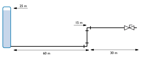
Locate the Coordinates section. In the table, enter the following settings:
Materials
Now add Water from the Material Library. The material properties will apply to the entire model domain by default.
Add Material
1
In the Materials toolbar, click  Add Material to open the Add Material window.
2
Go to the Add Material window.
3
In the tree, select Built-in > Water, liquid.
4
Click the Add to Component button in the window toolbar.
5
In the Materials toolbar, click  Add Material to close the Add Material window.
Materials
Water, liquid (mat1)
Click the  Zoom Extents button in the Graphics toolbar.
Pipe Flow (pfl)
Next, specify the dimensions and surface roughness of the pipe. Note that you can add multiple Pipe Properties features and assign them to different parts of a pipe network, should you have a system of made up of pipes with different characteristics.
Pipe Properties 1
1
In the Model Builder window, under Component 1 (comp1) > Pipe Flow (pfl) click Pipe Properties 1.
2
In the Settings window for Pipe Properties, locate the Pipe Shape section.
3
4
In the di text field, type Dh.
5
Locate the Flow Resistance section. From the Surface roughness list, choose Galvanized iron (0.15 mm).
Inlet 1
Set boundary conditions for the inlet and use a Volume Force feature to take gravity effects into account.
1
In the Physics toolbar, click  Points and choose Inlet.
2
In the Settings window for Inlet, locate the Inlet Specification section.
3
From the Specification list, choose Reservoir.
4
In the pres text field, type 101325[Pa]+H0*g_const*pfl.rho.
5
6
From the Entrance type list, choose Rounded (K = 0.05).
Volume Force 1
1
In the Physics toolbar, click  Boundaries and choose Volume Force.
2
The default volume force is a gravity vector pointing in the negative y direction (downward).
3
Click the  Zoom Extents button in the Graphics toolbar.
Next, add a number of point features to include the energy losses due to bends and the ball valve. The valve point may be difficult to select graphically with the mouse. Here, you can use the Selection list, as help to browse the points in a list.
Bend 1
1
In the Physics toolbar, click  Points and choose Bend.
2
Valve 1
1
In the Physics toolbar, click  Points and choose Valve.
2
3
In the Settings window for Valve, locate the Valve Specification section.
4
From the Valve list, choose Ball valve (K = 4.5).
To help graphically indicate locations of pipe network elements, the physics symbols are available.
5
In the Model Builder window, click Pipe Flow (pfl).
6
In the Settings window for Pipe Flow, locate the Physics Symbols section.
7
Select the Enable physics symbols checkbox.
8
Find the Show or hide all physics symbols subsection. Click Select All to display physics symbols for all features.
Study 1
The model is now ready for solving. Lower the default tolerance to increase the accuracy of the solution.
Step 1: Stationary
1
In the Model Builder window, under Study 1 click Step 1: Stationary.
2
In the Settings window for Stationary, locate the Study Settings section.
3
From the Tolerance list, choose User controlled.
4
In the Relative tolerance text field, type 1e-6.
5
In the Study toolbar, click  Compute.
Results
Pressure (pfl)
Default plots show the pressure drop in the pipe system, and the direction and velocity of the flow (Figure 2 and Figure 3). Modify the last plot to evaluate the Reynolds number and flow rate.
Velocity (pfl)
In the Model Builder window, expand the Results > Velocity (pfl) node.
Color Expression 1
1
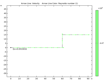
In the Model Builder window, expand the Results > Velocity (pfl) > Arrow Line 1 node, then click Color Expression 1.
2
In the Settings window for Color Expression, click Replace Expression in the upper-right corner of the Expression section. From the menu, choose Component 1 (comp1) > Pipe Flow > pfl.Re - Reynolds number - 1.
3
Click to expand the Title section. From the Title type list, choose Automatic.
Annotation 1
1
In the Model Builder window, right-click Velocity (pfl) and choose Annotation.
2
In the Settings window for Annotation, locate the Annotation section.
3
Click  Replace Expression.
4
Click thebutton. From the menu, choose Component 1 (comp1) > Pipe Flow > pfl.Qv - Volumetric flow rate magnitude - m³/s.
5
In the Text text field, type Qv=eval(pfl.Qv).
6
In the Velocity (pfl) toolbar, click  Plot.
7
Click the  Zoom Extents button in the Graphics toolbar.