PDF

Tubular Centrifuge
Introduction
A tubular centrifuge is a type of centrifugal separation device that is often used for separation of very fine solid particles from a liquid. It can be run in both a continuous and batch type configurations. The device usually consists of a cylindrical rotating bowl with a large aspect ratio where its length is often many times larger than the radius. The bowl has an inlet feed and an outlet.
The particle–liquid mixture enters the rotating bowl through the inlet feed. The large rotation speed of the bowl induces centrifugal forces on the particles which cause them to sediment near the inner walls of the bowl as long as the particle has a larger density compared to the fluid. The sedimentation rate depends on the particle densities and the rotation speeds. Larger rotation speeds enhance the sedimentation rate. Further, the particles with larger densities tend to sediment faster. This dependence on the particle densities can lead to a preferential sedimentation along the axial direction with the most dense particles sedimenting close to the inlet, while the less dense particles sediment at a larger axial distance from the inlet.
This model also demonstrates the process of restarting particle tracing simulations whereby the information of the particles from one study step is used as the initial conditions for a subsequent study step.
Model Definition
The geometry consists of a cylinder of radius 20 mm and a height of 225 mm. There is a circular inlet of radius 5 mm on end of the cylinder through which the particle-fluid mixture enters the cylinder. The mixture exits the cylinder through a circular outlet of radius 5 mm on the face opposite to the inlet. The geometry as presented in Figure 1 shows the cylinder and the outlet.
The particle-fluid mixture sample used in this model is water containing spherical particles of a fixed diameter of 20 μm. The sample contains three types of particles with densities of 1200, 1500, and 2200 kg/m3. The sample enters the inlet at a flow rate of 2.5 l/min. The fluid entering the cylinder faces a sudden expansion and the corresponding Reynolds number suggests that the flow is turbulent. This model solves the Reynolds-Averaged Navier–Stokes equations and uses the standard k-ω turbulence model to account for the turbulent fluid flow.
The cylinder rotates with an angular speed of 1000 rad/s. The effect of rotation on the fluid flow is modeled using a Rotating Domain feature. It is assumed that fluid velocities are stationary and thus the Frozen Rotor with Initialization study step is utilized to account for the rotational effects via the inclusion centrifugal and Coriolis forces. Similarly, the rotational effects on the particle motion are included via the Rotating Frame feature which adds these fictitious forces to the particles. The Gravity feature is used to apply gravitational force in the z direction. Drag forces are applied in entire domain using the Drag Force feature. Inertial effects due to the virtual mass and pressure gradient contributions are also included in the drag force calculations. A Time Dependent study step is used to solve the particle trajectories for a total simulation time of 2 s.
Figure 1: Model geometry of a tubular centrifuge device.
Notes on COMSOL Implementation
The model is solved in two steps. First, the fluid velocity and pressure are solved using the Turbulent Flow, k-ω interface and Frozen Rotor with Initialization study step. Then the particle trajectories are solved for using the Particle Tracing for Fluid Flow interface and Time Dependent study step.
A total of 3000 particles are released having a fixed diameter of 20 μm. The particle densities are equally distributed over 1200, 1500 and 2200 kg/m3. The particles are released along the inlet boundary with number density proportional to the fluid velocity along the axial direction. The Freeze wall condition is applied at the all the remaining boundaries to represent the sedimentation of the particles on the cylinder walls.
The rotational effects on the fluid and the particles can be accounted for by solving the equations of motion in either the lab-fixed (inertial) frame of reference or a (noninertial) reference frame attached to the cylinder. The analysis in the inertial reference frame would include solving the appropriate equations along with a moving mesh, which can be achieved via the Rotating Domain feature. However, the moving mesh computations can be computationally expensive in 3D, especially at large rotational speeds such as those of interest in this example. This can be avoided in situations where the geometry is rotationally invariant about the rotation axis, and the fluid flow is expected to be stationary in the spatial frame. In such situations, the model analysis is best suited in the noninertial reference frame, whereby the rotational effects are included via the addition of fictitious forces such as the centrifugal and the Coriolis forces.
For the fluid flow, this is easily achieved using the Frozen Rotor with Initialization study step. For the particle motion, the Particle Tracing Module contains the Rotating Frame feature that transforms the coordinate system from the lab-fixed inertial frame to the rotating noninertial frame and includes the fictitious force contributions to the forces on the particles. Since the coordinate system is now attached to a rotating frame, the mesh movement has to be disabled. This is achieved by disabling the Rotating Domain feature via the Modify model configuration for study step option in the Time Dependent study step used to compute the particle trajectories.
The particle trajectories are computed for a total simulation time of 2 seconds. This is split into two Time Dependent study steps, with the particle data from the final time step of the first study step being used as the initial conditions for the second study step. In order to accomplish this, it is essential that the Store particle status data checkbox is selected in the physics interface settings. The solutions from the two studies are then combined into one solution using the Combine Solutions study step.
Note that the particle tracing for an overall simulation time of 2 seconds can also be achieved directly in one study step. This is split into two study steps in this model to demonstrate the technique of restarting the particle tracing simulations and combining the solutions from two studies.
Results and Discussion
Figure 2 shows the velocity field (z direction) and the streamlines. The streamlines are colored based on the z-component of the fluid velocity. As the flow is fully developed, the velocity at center of the inlet is higher. The sudden expansion in the geometry causes the fluid velocity in the axial direction to drop immediately after the inlet. The rotational effects are clearly evident in the streamlines.
Figure 2: Velocity field and streamlines for the fluid flow.
Figure 3 show the particle trajectories at the end of 2 s. The particles are colored by their densities. The fluid carries the particles toward the outlet, while the centrifugal forces push the particles toward the cylinder walls. Denser particles are carried by the water for shorter distances and end up sedimenting closer to the inlet, while the less dense particles are carried further along. A large portion of the particles with the lowest density are found to sediment close to the outlet.
This preferential sedimentation is visualized in Figure 4, where the distribution of particle densities as a function of their z-coordinate is plotted at the end of 2 s. Finally, Figure 5 shows the number of particles sedimented on the walls as a function of time for each particle type. This illustrates the dependence of the sedimentation rates on the particle density.
Figure 3: Particle trajectories colored by particle diameter.
Figure 4: 1D histogram showing the distribution of particle densities collected at the wall as a function of the z-coordinate.
Figure 5: Number of sedimented particles as a function of time.
Application Library path: Particle_Tracing_Module/Fluid_Flow/tubular_centrifuge
Modeling Instructions
From the File menu, choose New.
New
In the New window, click  Model Wizard.
Model Wizard
1
In the Model Wizard window, click  3D.
2
In the Select Physics tree, select Fluid Flow > Single-Phase Flow > Turbulent Flow > Turbulent Flow, k-ω (spf).
3
Click Add.
4
In the Select Physics tree, select Mathematics > Deformed Mesh > Moving Mesh > Rotating Domain.
5
Click Add.
6
In the Select Physics tree, select Fluid Flow > Particle Tracing > Particle Tracing for Fluid Flow (fpt).
7
Click Add.
8
Click  Study.
9
In the Select Study tree, select Preset Studies for Some Physics Interfaces > Frozen Rotor with Initialization.
10
Global Definitions
Parameters 1
1
In the Model Builder window, under Global Definitions click Parameters 1.
2
In the Settings window for Parameters, locate the Parameters section.
3
Geometry 1
Cylinder 1 (cyl1)
1
In the Geometry toolbar, click  Cylinder.
2
In the Settings window for Cylinder, locate the Size and Shape section.
3
In the Radius text field, type R_tube.
4
In the Height text field, type L_tube.
5
Click  Build Selected.
Work Plane 1 (wp1)
In the Geometry toolbar, click  Work Plane.
Work Plane 1 (wp1) > Plane Geometry
In the Model Builder window, click Plane Geometry.
Work Plane 1 (wp1) > Circle 1 (c1)
1
In the Work Plane toolbar, click  Circle.
2
In the Settings window for Circle, locate the Size and Shape section.
3
In the Radius text field, type R_feed.
4
Click  Build Selected.
Work Plane 2 (wp2)
1
In the Model Builder window, under Component 1 (comp1) > Geometry 1 right-click Work Plane 1 (wp1) and choose Duplicate.
2
In the Settings window for Work Plane, locate the Plane Definition section.
3
In the z-coordinate text field, type L_tube.
Form Union (fin)
1
In the Geometry toolbar, click  Build All.
2
Click the  Transparency button in the Graphics toolbar.
Definitions
Create explicit selections for the inlet, outlet and the walls of the cylinder.
Inlet
1
In the Definitions toolbar, click  Explicit.
2
In the Settings window for Explicit, type Inlet in the Label text field.
3
Locate the Input Entities section. From the Geometric entity level list, choose Boundary.
4
Outlet
1
In the Definitions toolbar, click  Explicit.
2
In the Settings window for Explicit, type Outlet in the Label text field.
3
Locate the Input Entities section. From the Geometric entity level list, choose Boundary.
4
Walls
1
In the Definitions toolbar, click  Explicit.
2
In the Settings window for Explicit, type Walls in the Label text field.
3
Locate the Input Entities section. From the Geometric entity level list, choose Boundary.
4
Add Material
1
In the Materials toolbar, click  Add Material to open the Add Material window.
2
Go to the Add Material window.
3
In the tree, select Built-in > Water, liquid.
4
Click the Add to Component button in the window toolbar.
5
In the Materials toolbar, click  Add Material to close the Add Material window.
Now specify the settings for the Rotating Domain feature which usually controls the moving mesh. Even though this model solves the governing equations (for both the fluid and the particles) in a noninertial reference frame and thus avoids the need for a moving mesh, this node is needed for the Frozen Rotor study step.
Moving Mesh
Rotating Domain 1
1
In the Settings window for Rotating Domain, locate the Rotation section.
2
From the Rotation type list, choose Specified rotational velocity.
3
In the ω text field, type omega.
Turbulent Flow, k-ω (spf)
1
In the Model Builder window, under Component 1 (comp1) click Turbulent Flow, k-ω (spf).
2
In the Settings window for Turbulent Flow, k-ω, locate the Physical Model section.
3
Select the Include gravity checkbox.
Inlet 1
1
In the Physics toolbar, click  Boundaries and choose Inlet.
2
In the Settings window for Inlet, locate the Boundary Selection section.
3
From the Selection list, choose Inlet.
4
Locate the Boundary Condition section. From the list, choose Fully developed flow.
5
Locate the Fully Developed Flow section. Click the Flow rate button.
6
In the V0 text field, type Vol_f.
Outlet 1
1
In the Physics toolbar, click  Boundaries and choose Outlet.
2
In the Settings window for Outlet, locate the Boundary Selection section.
3
From the Selection list, choose Outlet.
4
Locate the Pressure Conditions section. Select the Normal flow checkbox.
Particle Tracing for Fluid Flow (fpt)
1
In the Model Builder window, under Component 1 (comp1) click Particle Tracing for Fluid Flow (fpt).
2
In the Settings window for Particle Tracing for Fluid Flow, locate the Additional Variables section.
3
Select the Store particle status data checkbox. This is necessary to use the particle trajectories from one study step as initial conditions for a subsequent study step.
Particle Properties 1
1
In the Model Builder window, under Component 1 (comp1) > Particle Tracing for Fluid Flow (fpt) click Particle Properties 1.
2
In the Settings window for Particle Properties, locate the Particle Properties section.
3
From the ρp list, choose User defined. In the associated text field, type 1200[kg/m^3].
4
In the dp text field, type dia_part.
Particle Properties 2
1
In the Physics toolbar, click  Global and choose Particle Properties.
2
In the Settings window for Particle Properties, locate the Particle Properties section.
3
From the ρp list, choose User defined. In the associated text field, type 1500[kg/m^3].
4
In the dp text field, type dia_part.
Particle Properties 3
1
Right-click Particle Properties 2 and choose Duplicate.
2
In the Settings window for Particle Properties, locate the Particle Properties section.
3
In the ρp text field, type 2200[kg/m^3].
Rotating Frame 1
1
In the Physics toolbar, click  Domains and choose Rotating Frame.
2
In the Settings window for Rotating Frame, locate the Rotating Frame section.
3
In the Ω text field, type omega.
Drag Force 1
1
In the Physics toolbar, click  Domains and choose Drag Force.
2
3
In the Settings window for Drag Force, locate the Drag Force section.
4
From the Drag law list, choose Schiller–Naumann.
5
From the u list, choose Velocity field (spf).
6
Locate the Additional Terms section. Select the Include virtual mass and pressure gradient forces checkbox. This is important to capture the inertial effects of the particle.
Gravity Force 1
1
In the Physics toolbar, click  Domains and choose Gravity Force.
2
Inlet 1
Release the particles such that number density of the particles is proportional to the axial component of the fluid density at the inlet. The fluid velocity at the inlet is used to initialize the particle velocities. Note that since the fluid velocity is defined in an inertial reference frame and the particle velocities are defined in the rotating (noninertial) reference frame, the moving frame velocity must be subtracted from the fluid velocity.
1
In the Physics toolbar, click  Boundaries and choose Inlet.
2
In the Settings window for Inlet, locate the Boundary Selection section.
3
From the Selection list, choose Inlet.
4
Locate the Initial Position section. From the Initial position list, choose Density.
5
In the N text field, type num_rel.
6
In the ρ text field, type w.
7
Locate the Initial Velocity section. From the u list, choose Velocity field (spf).
8
Click to expand the Advanced Settings section. Select the Subtract moving frame velocity from initial particle velocity checkbox.
Inlet 2
1
Right-click Inlet 1 and choose Duplicate.
2
In the Settings window for Inlet, click to expand the Released Particle Properties section.
3
From the Released particle properties list, choose Particle Properties 2.
Inlet 3
1
Right-click Inlet 2 and choose Duplicate.
2
In the Settings window for Inlet, locate the Released Particle Properties section.
3
From the Released particle properties list, choose Particle Properties 3.
Outlet 1
1
In the Physics toolbar, click  Boundaries and choose Outlet.
2
In the Settings window for Outlet, locate the Boundary Selection section.
3
From the Selection list, choose Outlet.
Particle Counter 1
1
In the Physics toolbar, click  Boundaries and choose Particle Counter.
2
In the Settings window for Particle Counter, locate the Boundary Selection section.
3
From the Selection list, choose Walls.
4
Locate the Particle Counter section. From the Particle selection list, choose Particle properties.
5
From the Released particle properties list, choose Particle Properties 1.
Particle Counter 2
1
Right-click Particle Counter 1 and choose Duplicate.
2
In the Settings window for Particle Counter, locate the Particle Counter section.
3
From the Released particle properties list, choose Particle Properties 2.
Particle Counter 3
1
Right-click Particle Counter 2 and choose Duplicate.
2
In the Settings window for Particle Counter, locate the Particle Counter section.
3
From the Released particle properties list, choose Particle Properties 3.
Add a Time Dependent study step to follow the Frozen Rotor study step. This study step only solves for the Particle Tracing for Fluid Flow interface. Further, since the usage of the Rotating Frame feature removes the need for a moving mesh, the Rotating Domain feature must be disabled for this study step.
Study 1
Step 3: Time Dependent
1
In the Study toolbar, click  Time Dependent.
2
In the Settings window for Time Dependent, locate the Study Settings section.
3
In the Output times text field, type range(0,0.05,1.0).
4
Locate the Physics and Variables Selection section. In the Solve for column of the table, under Component 1 (comp1), clear the checkboxes for Moving Mesh and Turbulent Flow, k-ω (spf).
5
Select the Modify model configuration for study step checkbox.
6
In the tree, select Component 1 (comp1) > Moving Mesh, Controls spatial frame > Rotating Domain 1.
7
Click  Disable.
8
Click to expand the Values of Dependent Variables section. Find the Values of variables not solved for subsection. From the Settings list, choose User controlled.
9
From the Method list, choose Solution.
10
From the Study list, choose Study 1, Frozen Rotor.
11
In the Study toolbar, click  Compute.
Results
Multislice 1
1
In the Model Builder window, expand the Velocity (spf) node, then click Multislice 1.
2
In the Settings window for Multislice, locate the Expression section.
3
In the Expression text field, type w.
4
Locate the Multiplane Data section. Find the x-planes subsection. In the Planes text field, type 0.
5
Find the y-planes subsection. In the Planes text field, type 0.
6
Find the z-planes subsection. From the Entry method list, choose Coordinates.
7
In the Coordinates text field, type range(0,(L_tube-0)/9,L_tube).
8
Locate the Coloring and Style section. From the Color table list, choose Prism.
Velocity (spf)
In the Velocity (spf) toolbar, click  Streamline.
Streamline 1
1
In the Settings window for Streamline, locate the Streamline Positioning section.
2
From the Positioning list, choose Starting-point controlled.
3
In the Points text field, type 100.
4
In the Velocity (spf) toolbar, click  Plot.
Color Expression 1
1
In the Velocity (spf) toolbar, click  Color Expression.
2
In the Settings window for Color Expression, locate the Expression section.
3
In the Expression text field, type w.
4
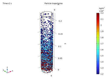
Locate the Coloring and Style section. Clear the Color legend checkbox. The plot should look like Figure 2.
Particle Trajectories (fpt)
1
In the Model Builder window, expand the Results > Particle Trajectories (fpt) node, then click Particle Trajectories (fpt).
2
In the Settings window for 3D Plot Group, locate the Color Legend section.
3
Select the Show units checkbox.
Particle Trajectories 1
1
Click the  Transparency button in the Graphics toolbar.
2
In the Model Builder window, click Particle Trajectories 1.
3
In the Settings window for Particle Trajectories, locate the Coloring and Style section.
4
Find the Point style subsection.
5
Select the Radius scale factor checkbox. In the associated text field, type 1.5.
6
In the Particle Trajectories (fpt) toolbar, click  Plot.
Color Expression 1
1
In the Model Builder window, expand the Particle Trajectories 1 node, then click Color Expression 1.
2
In the Settings window for Color Expression, locate the Expression section.
3
In the Expression text field, type fpt.rhop.
4
In the Particle Trajectories (fpt) toolbar, click  Plot.
The particles have not yet been fully separated from the fluid. In order to simulate the particle trajectories for an additional 1 second, it is possible to utilize the current solution as the initial conditions for a subsequent study step.
Add Study
1
In the Home toolbar, click  Add Study to open the Add Study window.
2
Go to the Add Study window.
3
Find the Studies subsection. In the Select Study tree, select General Studies > Time Dependent.
4
Click the Add Study button in the window toolbar.
5
In the Home toolbar, click  Add Study to close the Add Study window.
Study 2
Step 1: Time Dependent
1
In the Settings window for Time Dependent, locate the Study Settings section.
2
In the Output times text field, type range(1.0,0.05,2.0).
3
Locate the Physics and Variables Selection section. In the Solve for column of the table, under Component 1 (comp1), clear the checkboxes for Moving Mesh and Turbulent Flow, k-ω (spf).
4
Select the Modify model configuration for study step checkbox.
5
In the tree, select Component 1 (comp1) > Moving Mesh, Controls spatial frame > Rotating Domain 1.
6
Click  Disable.
7
Locate the Values of Dependent Variables section. Find the Initial values of variables solved for subsection. From the Settings list, choose User controlled.
8
From the Method list, choose Solution.
9
From the Study list, choose Study 1, Time Dependent.
10
From the Time (s) list, choose Last.
11
Find the Values of variables not solved for subsection. From the Settings list, choose User controlled.
12
From the Method list, choose Solution.
13
From the Study list, choose Study 1, Time Dependent.
14
In the Study toolbar, click  Compute.
Results
Particle Trajectories (fpt) 1
Now combine the solutions from the two particle tracing study steps into one solution. The solution at the first timestep in the Study 2 should be deleted while concatenating the two solutions.
Add Study
1
In the Home toolbar, click  Add Study to open the Add Study window.
2
Go to the Add Study window.
3
Find the Studies subsection. In the Select Study tree, select Empty Study.
4
Click the Add Study button in the window toolbar.
5
In the Home toolbar, click  Add Study to close the Add Study window.
Study 3
Step 1: Combine Solutions
1
In the Study toolbar, click  More Study Extensions and choose Combine Solutions.
2
In the Settings window for Combine Solutions, locate the Combine Solutions Settings section.
3
From the Solution operation list, choose Remove solutions.
4
From the Solution list, choose Study 2/Solution 4 (sol4).
5
From the Time (s) list, choose Manual.
Step 2: Combine Solutions 2
1
In the Study toolbar, click  More Study Extensions and choose Combine Solutions.
2
In the Settings window for Combine Solutions, locate the Combine Solutions Settings section.
3
From the First solution list, choose Study 1/Solution 1 (sol1).
4
In the Study toolbar, click  Compute.
Once the solutions from the two particle tracing studies are combined, create a new Particle dataset from the new solution.
Results
Particle 3
1
In the Results toolbar, click  More Datasets and choose Particle.
2
In the Settings window for Particle, locate the Particle Solution section.
3
From the Solution list, choose Solution 5 (sol5).
Particle Trajectories (fpt)
1
In the Model Builder window, under Results click Particle Trajectories (fpt).
2
In the Settings window for 3D Plot Group, locate the Data section.
3
From the Dataset list, choose Particle 3. The plot should look like Figure 3.
Animation 1
1
In the Results toolbar, click  Animation and choose Player.
2
In the Settings window for Animation, locate the Scene section.
3
From the Subject list, choose Particle Trajectories (fpt).
4
Locate the Frames section. From the Frame selection list, choose All.
5
Click the  Play button in the Graphics toolbar.
z histogram
1
In the Results toolbar, click  1D Plot Group.
2
In the Settings window for 1D Plot Group, type z histogram in the Label text field.
3
Locate the Data section. From the Dataset list, choose Particle 3.
4
From the Time selection list, choose Last.
5
Locate the Plot Settings section. Select the x-axis label checkbox.
6
Select the y-axis label checkbox.
7
In the x-axis label text field, type z [m].
8
In the y-axis label text field, type Count.
Histogram 1
1
In the z histogram toolbar, click  Histogram.
2
In the Settings window for Histogram, locate the Expression section.
3
In the Expression text field, type if(fpt.sidx==1,qz,0).
4
Select the Description checkbox. In the associated text field, type 1200[kg/m^3].
5
Locate the Bins section. From the Entry method list, choose Limits.
6
In the Limits text field, type range(0.01,(L_tube-0.01)/9,L_tube).
7
Locate the Output section. From the Function list, choose Discrete.
8
Click to expand the Coloring and Style section. From the Width list, choose 3.
9
Click to expand the Legends section. Select the Show legends checkbox.
10
Find the Include subsection. Clear the Solution checkbox.
11
Select the Description checkbox.
12
In the z histogram toolbar, click  Plot.
Histogram 2
1
Right-click Histogram 1 and choose Duplicate.
2
In the Settings window for Histogram, locate the Expression section.
3
In the Expression text field, type if(fpt.sidx==2,qz,0).
4
In the Description text field, type 1500[kg/m^3].
Histogram 3
1
Right-click Histogram 2 and choose Duplicate.
2
In the Settings window for Histogram, locate the Expression section.
3
In the Expression text field, type if(fpt.sidx==3,qz,0).
4
In the Description text field, type 2200[kg/m^3].
z histogram
1
In the Model Builder window, click z histogram.
2
In the z histogram toolbar, click  Plot. The plot should look like Figure 4.
Particle Counters
1
In the Results toolbar, click  1D Plot Group.
2
In the Settings window for 1D Plot Group, type Particle Counters in the Label text field.
3
Locate the Data section. From the Dataset list, choose Particle 3.
4
Locate the Plot Settings section. Select the x-axis label checkbox.
5
Select the y-axis label checkbox.
6
In the x-axis label text field, type Time (s).
7
In the y-axis label text field, type Number of stuck particles.
Global 1
1
In the Particle Counters toolbar, click  Global.
2
In the Settings window for Global, locate the y-Axis Data section.
3
4
Click to expand the Coloring and Style section. From the Width list, choose 3.
5
Click to expand the Legends section. In the Particle Counters toolbar, click  Plot. The plot should look like Figure 5.