PDF

Multipactor Saturation
Introduction
The multipactor effect is a sometimes deleterious phenomenon in which the number of electrons in a microwave cavity can grow exponentially. Free electrons within the cavity are accelerated by an RF signal, causing them to strike the cavity walls. If the electrons hit the walls with sufficient energy, the walls may then release secondary electrons. Under the right conditions, a single electron impact can cause the release of multiple secondary electrons, thus causing the total number of electrons in the cavity to increase.
If a certain relationship exists between the size of the cavity and the frequency and amplitude of the RF signal, then the electron emission occurs in resonance with the driving signal; the emitted secondary electrons are accelerated to the other end of the cavity, where they cause an even greater number of secondary electrons to be released, and so on.
When the number of electrons in the cavity becomes sufficiently large, then the mutual electrostatic repulsion between the electrons can disrupt their resonance with the driving RF signal, so that the total population of electrons does not grow without bound. Instead, the population of electrons eventually reaches a dynamic equilibrium in which the effects of space charge and the RF signal counterbalance each other. This verification model is a quasi-1D, two-way coupled particle field interaction model that shows how growth of space charge in a microwave cavity leads to multipactor saturation.
Model Definition
This example uses the Electrostatics interface to solve for the electric potential in a cavity and the Charged Particle Tracing interface to track electrons within the cavity. The RF voltage is applied by using the Ground boundary condition at one end of the geometry and the Electric Potential boundary condition at the other end, where the specified potential is a sinusoidal function of time,
where V0 (SI unit: V) is the amplitude of the signal and f (SI unit: 1/s) is the frequency.
The direction from the Ground boundary condition to the Electric Potential boundary condition is taken to be the positive x direction. Let D (SI unit: m) represent the gap thickness, the perpendicular distance between these two surfaces. The dimensions of the cavity in the y and z directions are assumed to be much larger than in the x direction. In addition, a constant, uniform magnetic field is applied within the cavity,
Multipaction can occur for specific combinations of the values of D, V0, f, and B0. This can include situations in which B0 = 0. A stability analysis of such a one-dimensional cavity geometry is demonstrated in Ref. 1. The model parameters used in this example are also based on Ref. 1: V0 = 1078 V, B0 = 360 G, f = 2.5 GHz, and D = 0.16 cm.
When an electron hits the wall at either end of the microwave cavity, the incident electron is removed from the simulation using a Wall node with the Disappear wall condition. Depending on the kinetic energy of the incident particle, it may release one or more secondary particles into the domain using the Secondary Emission subnode. The relationship between the kinetic energy of the incident particle and the number of emitted secondary electrons to release is called the secondary electron yield or SEY, an energy-dependent expression also from Ref. 1 and plotted in Figure 1,
Figure 1: Secondary electron yield (SEY) as a function of incident electron kinetic energy.
Although the model geometry in this example is three-dimensional, the model is essentially 1D-3V, meaning that only one component of particle position and all three components of the particle velocity are relevant. The spatial density of particles and the electric potential are assumed to be completely uniform in the y and z directions. To enforce this uniformity without introducing spurious y- and z-components of the electric field, a highly structured mesh was used with only a single element in these directions and a large number of very thin elements in the x direction, as shown in Figure 2.
Figure 2: Structured mesh to simulate the multipactor as a 1D-3V model.
To account for space-charge-induced debunching, in which the mutual electrostatic repulsion of electrons causes some of the model particles to slow down before hitting the wall (and thus release fewer secondary electrons), the particles were bidirectionally coupled to the electric potential in the cavity via the Electric Particle Field Interaction multiphysics coupling. At every time step, each model particle contributes to a volumetric space charge density term within the domain mesh element that it occupies, and then the electric potential is updated based on this space charge density term. Because the mesh only has a single element in the y and z directions, and the space charge density of particles is considered uniform within each mesh element, this method of coupling the particles and field does not introduce any y- or z-components of the electric field.
The actual number of electrons in the multipactor can be very large, so to reduce the computational cost a macroparticle-based approach was implemented. Each model particle represents n electrons for the purpose of computing the volumetric space charge density, where in this example n = 50,000. This value is entered into the Charge Multiplication Factor text field in the settings for the Electric Particle Field Interaction multiphysics coupling node. To check that the model is statistically converged, consider recomputing with a lower value of n, such as 10,000. This might require an increase in the Maximum number of secondary particles (see below), but the total charge of particles hitting the cavity walls should be unaffected if the model is statistically converged (see Figure 3).
The secondary electron yield is a continuous function of energy and is usually not integer-valued. For instance, consider a value of 2.4. In this scenario the Wall boundary condition has been configured to always release two secondary electrons, and to release a third electron with a 40% probability. For this reason, each Wall node has two Secondary Emission attributes, one for a whole number of guaranteed secondary electrons, and one for an additional secondary electron with an emission probability between 0 and 1.
It is important to allocate a sufficiently large number of secondary particles so that all of the secondary electron emission in the model can be simulated. The Maximum number of secondary particles can be controlled in the physics interface Particle Release and Propagation section. Because electrons are constantly added to and removed from the simulation domain, it is highly beneficial to recycle the degrees of freedom associated with the removed model particles. In the physics interface Advanced Settings section, the option All disappeared particles was selected from the Reuse particle degrees of freedom list. The default behavior is not to recycle degrees of freedom so that every emitted secondary particle has a unique index, but at the cost of significantly more DOFs overall.
The constant, spatially uniform magnetic field was applied using the Magnetic Force node. Because the particles in this example are nonrelativistic, the contribution of the moving electrons to the background magnetic field was deemed negligible.
The length of the simulation domain in the y and z directions should not affect the solution, so any length can be selected that allows the solution to be viewed easily in the Graphics window. When a particle hits one of the surfaces parallel to the xy- or zx-planes, the particle is immediately moved to the opposite face and then carries on with its precollision velocity. Particles can be mapped from a source boundary to a destination boundary using the Periodic Condition feature. This example uses a pair of Periodic Condition nodes, one for the two surfaces parallel to the xy-plane and another for the two surfaces parallel to the zx-plane.
Results and Discussion
The total charge of impacting particles on the cavity walls per half period is plotted over 20 RF cycles in Figure 3. Compare this figure to Figure 6a in Ref. 1.
After saturation has been reached, two distinct populations of electron can be observed by carefully inspecting every frame of the default Particle Trajectories plot. For many electrons, after being released from one wall, they are accelerated enough so that they hit the opposite wall about half of one RF cycle later. For some other particles, the trajectory is sufficiently curved by the magnetic field that they do not reach the opposite wall before the RF signal reverses direction, so they are instead accelerated back toward the wall that released them.
Another way to observe the behavior after saturation is to plot and animate the distribution of space charge density in a Slice plot through the model geometry. Figure 4 shows one such plot at a time after saturation has been reached. The dark band is the main band containing most of the newly released secondary electrons. The lighter band includes some recently released secondary particles that lead or trail the main band due to space charge effects, as well as electrons that did not quite reach the opposite wall during the last RF cycle. The space charge density uses constant shape functions within each mesh element, so the sharp changes in color just indicate where one element ends and the next element begins. To make plot look smoother, consider refining the mesh in the x direction (which might also require a larger number of model particles for statistical convergence) or smoothing the solution during results processing.
You can also try animating either the Particle Trajectories plot or the Slice plot shown in Figure 4 to visualize how the band of maximum charge density moves in phase with the applied RF voltage.
Figure 3: Total charge of impacting electrons per unit area, per RF half-cycle.
Figure 4: Space charge density in a cross section of the model geometry after saturation.
Reference
1. S. Riyopoulos, “Multipactor saturation due to space-charge-induced debunching,” Phys. Plasmas, vol. 4, no. 5, pp. 1448–1462, 1997.
Application Library path: Particle_Tracing_Module/Charged_Particle_Tracing/multipactor_saturation
Modeling Instructions
From the File menu, choose New.
New
In the New window, click  Model Wizard.
Model Wizard
1
In the Model Wizard window, click  3D.
2
In the Select Physics tree, select AC/DC > Particle Tracing > Particle–Field Interaction, Nonrelativistic.
3
Click Add.
4
Click  Study.
5
In the Select Study tree, select Preset Studies for Selected Multiphysics > Time Dependent.
6
Global Definitions
Parameters 1
Load the model parameters from a file.
1
In the Model Builder window, under Global Definitions click Parameters 1.
2
In the Settings window for Parameters, locate the Parameters section.
3
Click  Load from File.
4
Variables 1
1
In the Home toolbar, click  Variables and choose Global Variables.
Load the global variables from a file.
2
In the Settings window for Variables, locate the Variables section.
3
Click  Load from File.
4
These global variables will be used to suppress the release of secondary electrons when the RF field exerts a force in the outward normal direction.
Piecewise 1 (pw1)
1
In the Home toolbar, click  Functions and choose Global > Piecewise.
2
In the Settings window for Piecewise, locate the Definition section.
3
Find the Intervals subsection. In the table, enter the following settings:
4
Locate the Units section. In the Arguments text field, type eV.
5
In the Function text field, type 1.
6
Click  Plot. Compare the resulting plot to Figure 1. This function will be used to define the secondary electron yield (SEY) as a function of the kinetic energy of the incident particle.
Geometry 1
1
In the Model Builder window, under Component 1 (comp1) click Geometry 1.
2
In the Settings window for Geometry, locate the Units section.
3
From the Length unit list, choose mm.
Block 1 (blk1)
1
In the Geometry toolbar, click  Block.
2
In the Settings window for Block, locate the Size and Shape section.
3
In the Width text field, type D.
4
In the Depth text field, type L.
5
In the Height text field, type L.
6
Click  Build All Objects.
Any value of L should work, since the geometry extends infinitely far in the y and z directions, so a value was chosen that allows the geometry to be viewed easily in the Graphics window.
Definitions
Variables 2
1
In the Definitions toolbar, click  Local Variables.
2
In the Settings window for Variables, locate the Variables section.
3
Click  Load from File.
4
Some of these variables will be used to define the number of released secondary electrons at the boundaries. Others are postprocessing variables that will be used to plot the number of electron impacts at the cavity walls over time. Note how the at operator is used to evaluate an expression at a previous solution time.
Electrostatics (es)
Ground 1
1
In the Physics toolbar, click  Boundaries and choose Ground.
2
Electric Potential 1
1
In the Physics toolbar, click  Boundaries and choose Electric Potential.
2
3
In the Settings window for Electric Potential, locate the Electric Potential section.
4
In the V0 text field, type V0*sin(2*pi*f0*t).
Next, allow Advanced Physics Options to be shown if they are not already shown. This is required to access the settings that govern recycling of degrees of freedom for the Charged Particle Tracing interface.
Root
1
Click the  Show More Options button in the Model Builder toolbar.
2
In the Show More Options dialog, in the tree, select the checkbox for the node Physics > Advanced Physics Options.
3
Charged Particle Tracing (cpt)
1
In the Model Builder window, under Component 1 (comp1) click Charged Particle Tracing (cpt).
2
In the Settings window for Charged Particle Tracing, locate the Particle Release and Propagation section.
3
From the Particle release specification list, choose Specify release times.
4
In the Maximum number of secondary particles text field, type 1000.
5
Click to expand the Advanced Settings section. From the Reuse particle degrees of freedom list, choose All disappeared particles.
Electric Force 1
1
In the Model Builder window, under Component 1 (comp1) > Charged Particle Tracing (cpt) click Electric Force 1.
2
In the Settings window for Electric Force, locate the Electric Force section.
3
From the E list, choose Electric field (es/fsp1).
Magnetic Force 1
1
In the Physics toolbar, click  Domains and choose Magnetic Force.
2
3
In the Settings window for Magnetic Force, locate the Magnetic Force section.
4
Specify the B vector as
Release from Grid 1
1
In the Physics toolbar, click  Global and choose Release from Grid.
2
In the Settings window for Release from Grid, locate the Initial Coordinates section.
3
In the qx,0 text field, type range(0.01,0.02,0.99)*D.
4
In the qy,0 text field, type L/2.
5
In the qz,0 text field, type L/2.
The initial particle positions are distributed across the width of the cavity so that at least some of these seed charges will hit the walls at sufficiently high energy to start the electron avalanche.
Next, two Secondary Emission nodes will be added to Wall nodes on opposite sides of the cavity. The first releases a guaranteed number of secondary electrons equal to the largest integer less than the secondary electron yield. The second releases one more electron with a probability based on the remainder of the secondary electron yield. Two Wall nodes have been used because each has an additional requirement that the force from the RF signal should point into the simulation domain, or else no particles can be released.
Wall 2
1
In the Physics toolbar, click  Boundaries and choose Wall.
2
3
In the Settings window for Wall, locate the Wall Condition section.
4
From the Wall condition list, choose Disappear.
Secondary Emission 1
1
In the Physics toolbar, click  Attributes and choose Secondary Emission.
2
In the Settings window for Secondary Emission, locate the Secondary Particles section.
3
In the Ns text field, type SEY_int_left.
4
From the Initial velocity list, choose Thermal.
5
In the T text field, type T0.
Secondary Emission 2
1
Right-click Secondary Emission 1 and choose Duplicate.
2
In the Settings window for Secondary Emission, locate the Secondary Emission Condition section.
3
From the Secondary emission condition list, choose Probability.
4
In the γ text field, type SEY_frac_left.
5
Locate the Secondary Particles section. In the Ns text field, type 1.
Wall 2
In the Model Builder window, click Wall 2.
Accumulator 1
1
In the Physics toolbar, click  Attributes and choose Accumulator.
2
In the Settings window for Accumulator, locate the Units section.
3
Click  Select Quantity.
4
In the Physical Quantity dialog, type surfacecharge in the text field.
5
In the tree, select Electromagnetics > Surface charge density (C/m^2).
6
7
In the Settings window for Accumulator, locate the Accumulator Settings section.
8
In the R text field, type e_const*n.
These accumulated variables will be used in results processing to track the total number of electron impacts on each surface over time.
Now duplicate this Wall boundary condition and apply the copy to the opposite wall, with the appropriate modifications.
Wall 3
1
Right-click Wall 2 and choose Duplicate.
2
Secondary Emission 1
1
In the Model Builder window, expand the Wall 3 node, then click Secondary Emission 1.
2
In the Settings window for Secondary Emission, locate the Secondary Particles section.
3
In the Ns text field, type SEY_int_right.
Secondary Emission 2
1
In the Model Builder window, click Secondary Emission 2.
2
In the Settings window for Secondary Emission, locate the Secondary Emission Condition section.
3
In the γ text field, type SEY_frac_right.
Periodic boundary conditions will be used on the remaining surfaces to represent the infinite extent of the cavity in the y and z directions. Each Periodic Condition node is applied to one pair of boundaries on opposite sides.
Periodic Condition 1
1
In the Physics toolbar, click  Boundaries and choose Periodic Condition.
2
Periodic Condition 2
1
In the Physics toolbar, click  Boundaries and choose Periodic Condition.
2
Multiphysics
Electric Particle–Field Interaction 1 (epfi1)
1
In the Model Builder window, under Component 1 (comp1) > Multiphysics click Electric Particle–Field Interaction 1 (epfi1).
2
In the Settings window for Electric Particle–Field Interaction, click to expand the Charge Multiplication Factor section.
3
In the n text field, type n.
This multiplication factor is the number of real electrons that are represented by each model particle for the purpose of computing the space charge density. This prevents an inordinate number of particle degrees of freedom from being required.
Mesh 1
A structured mesh will be designed with a single element in the y and z directions, but very fine resolution in the x direction in which the space charge density may vary greatly.
Mapped 1
1
In the Mesh toolbar, click  More Generators and choose Mapped.
2
Distribution 1
1
In the Mesh toolbar, click  Distribution.
2
3
In the Settings window for Distribution, locate the Distribution section.
4
In the Number of elements text field, type 1.
Swept 1
In the Mesh toolbar, click  Swept.
Distribution 1
1
In the Mesh toolbar, click  Distribution.
2
In the Settings window for Distribution, locate the Distribution section.
3
In the Number of elements text field, type 100.
4
Click  Build All. Compare the resulting plot to Figure 2.
Study 1
Now adjust the study settings to trace the particles for up to 20 RF cycles. A rather small time step is used in order to create higher-quality animations in postprocessing, but a larger time step could also be used to reduce file size.
Step 1: Time Dependent
1
In the Model Builder window, under Study 1 click Step 1: Time Dependent.
2
In the Settings window for Time Dependent, locate the Study Settings section.
3
In the Output times text field, type range(0,1/(100*f0),20/f0).
Solution 1 (sol1)
1
In the Study toolbar, click  Show Default Solver.
2
In the Model Builder window, expand the Solution 1 (sol1) node.
3
In the Model Builder window, expand the Study 1 > Solver Configurations > Solution 1 (sol1) > Time-Dependent Solver 1 node.
4
Right-click Study 1 > Solver Configurations > Solution 1 (sol1) > Time-Dependent Solver 1 and choose Fully Coupled.
5
In the Settings window for Fully Coupled, locate the General section.
6
From the Linear solver list, choose Direct.
7
In the Study toolbar, click  Compute.
If the Maximum number of secondary particles in the settings for the Charged Particle Tracing interface is too low, a warning might appear, saying that some secondary particles were not released. For the parameter values in these instructions, 1000 secondary particles is expected to suffice and this warning should not appear. If you later reduce the value of the model parameter n, the charge multiplication factor, then an increase in the preallocated secondary particles may be required.
Results
Some default plots, as well as a default Particle dataset, are created. These can be viewed at any time. To see the quantitative information that indicates whether saturation has been reached, create a 1D Plot Group to track the number of electron impacts over time.
1D Plot Group 5
In the Results toolbar, click  1D Plot Group.
Global 1
1
In the 1D Plot Group 5 toolbar, click  Global.
2
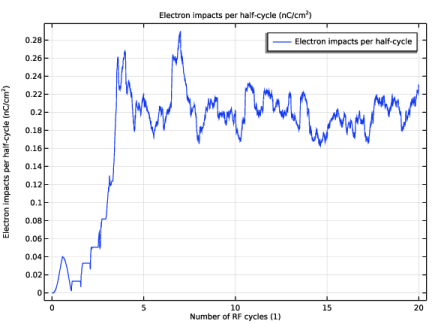
In the Settings window for Global, click Replace Expression in the upper-right corner of the y-Axis Data section. From the menu, choose Component 1 (comp1) > Definitions > Variables > impacts_change - Electron impacts per half-cycle - C/m².
3
Locate the y-Axis Data section. In the table, enter the following settings:
4
Locate the x-Axis Data section. From the Parameter list, choose Expression.
5
Click Replace Expression in the upper-right corner of the x-Axis Data section. From the menu, choose Global definitions > Variables > tau - Number of RF cycles - 1.
6
In the 1D Plot Group 5 toolbar, click  Plot. Compare the resulting plot to Figure 3.
Cut Plane 1
1
In the Results toolbar, click  Cut Plane.
2
In the Settings window for Cut Plane, locate the Plane Data section.
3
From the Plane list, choose xy-planes.
4
In the z-coordinate text field, type L/2.
5
Click  Plot, to verify that the cut plane passes through the middle of the domain.
2D Plot Group 6
1
In the Results toolbar, click  2D Plot Group.
2
In the Settings window for 2D Plot Group, locate the Data section.
3
From the Dataset list, choose Cut Plane 1.
Surface 1
1
In the 2D Plot Group 6 toolbar, click  Surface.
2
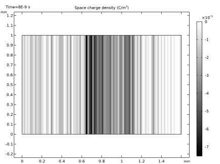
In the Settings window for Surface, click Replace Expression in the upper-right corner of the Expression section. From the menu, choose Component 1 (comp1) > Currents and charge > epfi1.rhos - Space charge density - C/m³.
3
Locate the Coloring and Style section. From the Color table list, choose GrayScale.
4
In the 2D Plot Group 6 toolbar, click  Plot. Compare the resulting plot to Figure 4.
Optionally, you may animate the Slice plot or the Particle Trajectories plot.
Animation 1
1
In the 2D Plot Group 6 toolbar, click  Animation and choose Player.
2
In the Settings window for Animation, locate the Frames section.
3
In the Number of frames text field, type 200.
4
Click the  Play button in the Graphics toolbar.