|
|
|

|
•
|
rp (SI unit: m) is the radius of a spherical particle in the field,
|
|
•
|
|
•
|
Erms (SI unit: V/m) is the root mean square electric field.
|

|
•
|
|
1
|
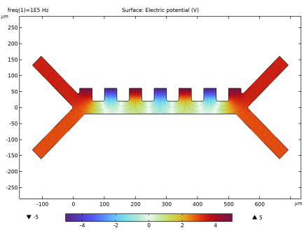
Study 1 (Stationary and Frequency Domain) solves for the fluid velocity, pressure, and AC electric potential.
|
|
2
|
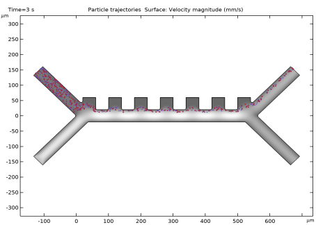
Study 2 (Time Dependent) estimates the particle trajectories in the flow without the DEP force, so that all particles (platelets and RBC) follow the same path.
|
|
3
|
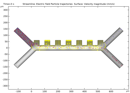
Study 3 (Time Dependent) computes the particle trajectories including the DEP force.
|
|
1
|
|
2
|
|
3
|
Click Add.
|
|
4
|
|
5
|
Click Add.
|
|
6
|
In the Select Physics tree, select Fluid Flow > Particle Tracing > Particle Tracing for Fluid Flow (fpt).
|
|
7
|
Click Add.
|
|
8
|
Click
|
|
1
|
|
2
|
Browse to the model’s Application Libraries folder and double-click the file dielectrophoretic_separation_geom_sequence.mph.
|
|
1
|
|
2
|
|
3
|
Click
|
|
4
|
Browse to the model’s Application Libraries folder and double-click the file dielectrophoretic_separation_parameters.txt.
|
|
1
|
|
2
|
|
3
|
|
1
|
|
2
|
|
3
|
|
1
|
|
3
|
|
4
|
|
1
|
|
3
|
|
4
|
|
1
|
|
1
|
|
2
|
In the Settings window for Particle Tracing for Fluid Flow, locate the Particle Release and Propagation section.
|
|
3
|
|
1
|
In the Model Builder window, under Component 1 (comp1) > Particle Tracing for Fluid Flow (fpt) click Particle Properties 1.
|
|
2
|
|
3
|
Locate the Particle Properties section. From the ρp list, choose User defined. In the associated text field, type rho_p.
|
|
4
|
|
1
|
|
2
|
|
3
|
Locate the Particle Properties section. From the ρp list, choose User defined. In the associated text field, type rho_p.
|
|
4
|
|
1
|
|
2
|
|
4
|
|
5
|
|
1
|
|
2
|
|
3
|
Click to expand the Released Particle Properties section. From the Released particle properties list, choose Red Blood Cells.
|
|
1
|
|
1
|
|
2
|
|
3
|
|
4
|
|
5
|
Locate the Additional Terms section. Select the Include virtual mass and pressure gradient forces checkbox.
|
|
1
|
|
2
|
In the Settings window for Dielectrophoretic Force, type Dielectrophoretic Force, Platelets in the Label text field.
|
|
3
|
|
4
|
|
5
|
Locate the Advanced Settings section. Select the Use piecewise polynomial recovery on field checkbox.
|
|
6
|
|
1
|
|
2
|
|
3
|
|
4
|
|
5
|
|
1
|
|
2
|
In the Settings window for Dielectrophoretic Force, type Dielectrophoretic Force, Red Blood Cells in the Label text field.
|
|
3
|
Locate the Advanced Settings section. From the Affected particle properties list, choose Red Blood Cells.
|
|
1
|
In the Model Builder window, expand the Dielectrophoretic Force, Red Blood Cells node, then click Shell 1.
|
|
2
|
|
3
|
|
4
|
|
5
|
|
1
|
In the Model Builder window, under Component 1 (comp1) > Particle Tracing for Fluid Flow (fpt) click Platelets.
|
|
2
|
|
3
|
|
4
|
|
1
|
|
2
|
|
3
|
|
4
|
|
1
|
In the Model Builder window, under Component 1 (comp1) right-click Materials and choose Blank Material.
|
|
2
|
|
1
|
|
2
|
Go to the Add Study window.
|
|
3
|
Find the Physics interfaces in study subsection. In the table, clear the Solve checkboxes for Electric Currents (ec) and Particle Tracing for Fluid Flow (fpt).
|
|
4
|
|
5
|
Click the Add Study button in the window toolbar.
|
|
6
|
|
1
|
|
2
|
|
3
|
|
4
|
|
1
|
|
2
|
|
1
|
|
2
|
|
3
|
|
1
|
|
2
|
Go to the Add Study window.
|
|
3
|
Find the Physics interfaces in study subsection. In the table, clear the Solve checkboxes for Electric Currents (ec) and Creeping Flow (spf).
|
|
4
|
|
5
|
Click the Add Study button in the window toolbar.
|
|
6
|
|
1
|
In the Model Builder window, under Study 2, no Dielectrophoretic Force click Step 1: Time Dependent.
|
|
2
|
|
3
|
|
4
|
Locate the Physics and Variables Selection section. Select the Modify model configuration for study step checkbox.
|
|
5
|
In the tree, select Component 1 (comp1) > Particle Tracing for Fluid Flow (fpt) > Dielectrophoretic Force, Platelets and Component 1 (comp1) > Particle Tracing for Fluid Flow (fpt) > Dielectrophoretic Force, Red Blood Cells.
|
|
6
|
Click
|
|
7
|
Click to expand the Values of Dependent Variables section. Find the Values of variables not solved for subsection. From the Settings list, choose User controlled.
|
|
8
|
|
9
|
|
10
|
|
1
|
|
2
|
Clear the Show legends checkbox.
|
|
1
|
In the Model Builder window, expand the Particle Trajectories (fpt) node, then click Particle Trajectories 1.
|
|
2
|
|
3
|
Find the Point style subsection. In the Point radius expression text field, type if(fpt.sidx==2,dp2/2,dp1).
|
|
1
|
In the Model Builder window, expand the Particle Trajectories 1 node, then click Color Expression 1.
|
|
2
|
|
3
|
|
4
|
|
1
|
|
2
|
In the Settings window for Surface, click Replace Expression in the upper-right corner of the Expression section. From the menu, choose Component 1 (comp1) > Creeping Flow > Velocity and pressure > spf.U - Velocity magnitude - m/s.
|
|
3
|
|
4
|
|
5
|
|
6
|
|
7
|
|
8
|
|
1
|
In the Model Builder window, under Study 2, no Dielectrophoretic Force click Step 1: Time Dependent.
|
|
2
|
|
3
|
Select the Plot checkbox.
|
|
4
|
|
5
|
|
1
|
|
2
|
Go to the Add Study window.
|
|
3
|
Find the Physics interfaces in study subsection. In the table, clear the Solve checkboxes for Electric Currents (ec) and Creeping Flow (spf).
|
|
4
|
|
5
|
Click the Add Study button in the window toolbar.
|
|
6
|
|
1
|
|
2
|
|
3
|
|
4
|
Locate the Values of Dependent Variables section. Find the Values of variables not solved for subsection. From the Settings list, choose User controlled.
|
|
5
|
|
6
|
|
7
|
|
1
|
|
2
|
Clear the Show legends checkbox.
|
|
1
|
In the Model Builder window, expand the Particle Trajectories (fpt) 1 node, then click Particle Trajectories 1.
|
|
2
|
|
3
|
Find the Point style subsection. In the Point radius expression text field, type if(fpt.dp==dp2,dp2/2,dp1).
|
|
1
|
In the Model Builder window, expand the Particle Trajectories 1 node, then click Color Expression 1.
|
|
2
|
|
3
|
|
4
|
|
1
|
|
2
|
In the Settings window for Surface, click Replace Expression in the upper-right corner of the Expression section. From the menu, choose Component 1 (comp1) > Creeping Flow > Velocity and pressure > spf.U - Velocity magnitude - m/s.
|
|
3
|
|
4
|
|
5
|
|
6
|
|
7
|
|
1
|
|
2
|
In the Settings window for Streamline, click Replace Expression in the upper-right corner of the Expression section. From the menu, choose Component 1 (comp1) > Electric Currents > Electric > ec.Ex,ec.Ey - Electric field.
|
|
3
|
|
4
|
|
5
|
|
6
|
Locate the Coloring and Style section. Find the Point style subsection. From the Color list, choose Yellow.
|
|
7
|
|
8
|
|
9
|
Drag and drop above Particle Trajectories 1.
|
|
10
|
|
1
|
|
2
|
|
3
|
Select the Plot checkbox.
|
|
4
|
|
5
|
|
1
|
|
1
|
|
2
|
|
1
|
|
2
|
|
3
|
|
4
|
|
5
|
|
1
|
|
2
|
|
3
|
|
4
|
|
5
|
|
6
|
|
7
|
|
1
|
|
2
|
Select the object r2 only.
|
|
3
|
|
4
|
|
5
|
|
6
|
|
1
|
|
2
|
Click in the Graphics window and then press Ctrl+A to select all objects.
|
|
3
|
|
4
|
Select the Keep input objects checkbox.
|
|
5
|
|
1
|
|
2
|
|
3
|
|
4
|
|
5
|
|
1
|
|
2
|
Select the object sq1 only.
|
|
3
|
|
4
|
|
5
|
|
1
|
|
2
|
Click in the Graphics window and then press Ctrl+A to select all objects.
|
|
3
|
|
4
|
Clear the Keep interior boundaries checkbox.
|
|
1
|
|
2
|
On the object uni1, select Points 5, 6, 8, 9, 11, 13, 15, 17, 19, 22, 24, 26, 28, 30, 32, 34, 35, and 37 only.
|
|
3
|
|
4
|
|
5
|
Click
|