
|
|
|
|
1
|
|
2
|
In the Application Libraries window, select Heat Transfer Module > Phase Change > superheated_steam_drying in the tree.
|
|
3
|
Click
|
|
1
|
|
2
|
|
1
|
|
2
|
|
3
|
|
4
|
From the Extrapolation list, choose Linear, because the tolerance of the bisection associated with the stop condition might cause the argument to be marginally outside the bounds.
|
|
5
|
|
6
|
|
7
|
|
8
|
Locate the Control Variable Discretization section. From the Control type list, choose Piecewise Bernstein polynomial.
|
|
9
|
|
10
|
|
11
|
Click OK.
|
|
12
|
|
13
|
Click
|
|
14
|
|
15
|
Click OK.
|
|
1
|
In the Model Builder window, expand the Component 1 (comp1) > Definitions > Shared Properties node, then click Ambient Properties 1 (ampr1).
|
|
2
|
|
3
|
|
4
|
|
1
|
|
2
|
|
3
|
|
1
|
|
2
|
|
3
|
|
1
|
|
2
|
|
1
|
|
2
|
Go to the Add Study window.
|
|
3
|
|
4
|
Click the Add Study button in the window toolbar.
|
|
5
|
|
6
|
Click the Add Study button in the window toolbar twice.
|
|
7
|
|
1
|
|
2
|
In the Solve for column of the table, under Component 1 (comp1), clear the checkboxes for Heat Transfer in Moist Air (ht) and Moisture Transport in Free and Porous Media (mt).
|
|
3
|
In the Solve for column of the table, under Component 1 (comp1) > Multiphysics, clear the checkboxes for Moisture Flow 1 (mf1), Heat and Moisture 1 (ham1), and Nonisothermal Flow 1 (nitf1).
|
|
4
|
In the Solve for column of the table, under Component 1 (comp1) > Definitions, clear the checkbox for Control Variables.
|
|
5
|
|
6
|
|
7
|
|
8
|
|
1
|
|
2
|
|
1
|
|
2
|
In the Solve for column of the table, under Component 1 (comp1), clear the checkbox for Laminar Flow (spf).
|
|
3
|
Click to expand the Values of Dependent Variables section. Find the Values of variables not solved for subsection. From the Settings list, choose User controlled.
|
|
4
|
|
5
|
|
6
|
Locate the Study Extensions section. In the table, click to select the cell at row number 1 and column number 2.
|
|
7
|
Click
|
|
8
|
Clear the Auxiliary sweep checkbox.
|
|
1
|
|
2
|
|
3
|
|
4
|
|
5
|
Click to expand the Solver Settings section. Find the Objective settings subsection. From the Objective scaling list, choose Initial solution based.
|
|
6
|
Click Add Expression in the upper-right corner of the Objective Function section. From the menu, choose Global definitions > Parameters > tmax - Final time - s.
|
|
7
|
|
8
|
|
9
|
|
11
|
Click Add Expression in the upper-right corner of the Constraints section. From the menu, choose Component 1 (comp1) > Definitions > Control Function 1 > comp1.cfunc1.avg - Control function average - K.
|
|
12
|
Click Add Expression in the upper-right corner of the Constraints section. From the menu, choose Component 1 (comp1) > Definitions > Nonlocal couplings > comp1.aveop1(expr) - Average 1.
|
|
13
|
Locate the Constraints section. In the table, enter the following settings:, so that the constraints are well scaled.
|
|
14
|
|
15
|
|
16
|
|
17
|
In the Study toolbar, click
|
|
1
|
|
2
|
|
3
|
|
4
|
|
5
|
|
6
|
|
1
|
|
2
|
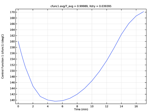
In the Settings window for Global, click Section toolbar in the upper-right corner of the y-Axis Data section. From the menu, choose Component 1 (comp1) > Definitions > Functions > cfunc1(s0) - Control Function 1 (cfunc1).
|
|
3
|
Locate the y-Axis Data section. In the table, enter the following settings:
|
|
1
|
In the Model Builder window, expand the Study 3: Optimal Control > Solver Configurations > Solution 3 (sol3) node, then click Optimization Solver 1.
|
|
2
|
|
3
|
Select the Move limits checkbox.
|
|
4
|
|
5
|
In the Model Builder window, expand the Study 3: Optimal Control > Solver Configurations > Solution 3 (sol3) > Optimization Solver 1 > Time-Dependent Solver 1 node, then click Advanced.
|
|
6
|
|
7
|
Clear the Reuse sparsity pattern checkbox to get a cleaner log.
|
|
1
|
|
2
|
|
3
|
Select the Plot checkbox.
|
|
5
|
|
1
|
|
2
|
In the Solve for column of the table, under Component 1 (comp1), select the checkbox for Laminar Flow (spf).
|
|
3
|
Click to expand the Values of Dependent Variables section. Find the Values of variables not solved for subsection. From the Method list, choose Solution.
|
|
4
|
|
5
|
Find the Initial values of variables solved for subsection. From the Settings list, choose User controlled.
|
|
6
|
|
7
|
|
8
|
|
9
|
|
10
|
|
11
|
Clear the Generate default plots checkbox.
|
|
12
|
|
13
|
|
1
|
|
2
|
|
3
|
|
4
|
|
5
|
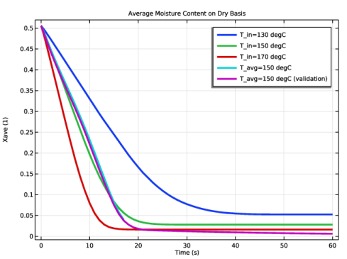
Locate the y-Axis Data section. In the table, enter the following settings:
|
|
6
|
|
7
|
Select the Description checkbox.
|
|
1
|
|
2
|
|
3
|
|
4
|
Locate the y-Axis Data section. In the table, enter the following settings:
|
|
5
|