|
|
|
|
1
|
|
2
|
In the Select Physics tree, select Structural Mechanics > Rotordynamics > Hydrodynamic Bearing (hdb).
|
|
3
|
Click Add.
|
|
4
|
Click
|
|
5
|
|
6
|
Click
|
|
1
|
|
2
|
|
3
|
Click
|
|
4
|
Browse to the model’s Application Libraries folder and double-click the file step_thrust_bearing_shape_optimization_parameters.txt.
|
|
1
|
|
2
|
|
3
|
|
4
|
|
5
|
Click to expand the Layers section. In the table, enter the following settings:
|
|
1
|
Right-click Component 1 (comp1) > Geometry 1 > Work Plane 1 (wp1) > Plane Geometry > Circle 1 (c1) and choose Duplicate.
|
|
2
|
|
3
|
|
4
|
|
1
|
Right-click Component 1 (comp1) > Geometry 1 > Work Plane 1 (wp1) > Plane Geometry > Circle 2 (c2) and choose Duplicate.
|
|
2
|
|
3
|
|
1
|
|
2
|
|
3
|
|
4
|
|
1
|
|
2
|
|
3
|
Click in the Graphics window and then press Ctrl+D to clear all objects.
|
|
4
|
|
5
|
|
6
|
|
7
|
|
8
|
Locate the Selections of Resulting Entities section. Select the Resulting objects selection checkbox.
|
|
9
|
Click
|
|
1
|
|
2
|
In the Settings window for Disk Selection, type Disk Selection: Leading Edge in the Label text field.
|
|
3
|
|
4
|
|
5
|
|
6
|
|
7
|
|
8
|
|
9
|
Click
|
|
1
|
|
2
|
|
3
|
|
4
|
|
5
|
Click
|
|
6
|
|
1
|
|
2
|
|
3
|
|
4
|
|
5
|
|
6
|
|
7
|
Click
|
|
8
|
|
1
|
|
2
|
|
3
|
|
4
|
|
5
|
Click
|
|
1
|
|
2
|
|
3
|
|
4
|
|
5
|
Click
|
|
6
|
|
1
|
|
2
|
|
3
|
|
4
|
|
5
|
In the Add dialog, select Disk Selection: Leading Edge (Work Plane 1) in the Selections to add list.
|
|
6
|
Click OK.
|
|
1
|
|
2
|
In the Settings window for Union Selection, type Trailing Edges of the Pads in the Label text field.
|
|
3
|
|
4
|
|
5
|
Click
|
|
6
|
Click
|
|
7
|
In the Add dialog, select Disk Selection: Trailing Edge (Work Plane 1) in the Selections to add list.
|
|
8
|
Click OK.
|
|
9
|
|
1
|
|
2
|
|
3
|
|
4
|
|
5
|
|
6
|
Click OK.
|
|
7
|
|
1
|
|
2
|
|
3
|
|
4
|
|
5
|
Click
|
|
6
|
Click
|
|
7
|
|
8
|
Click OK.
|
|
9
|
|
1
|
|
2
|
|
3
|
|
4
|
Click
|
|
5
|
|
6
|
Click OK.
|
|
7
|
|
8
|
|
9
|
|
1
|
|
2
|
|
3
|
|
4
|
|
5
|
Click
|
|
6
|
|
7
|
Click OK.
|
|
8
|
|
9
|
|
10
|
|
11
|
|
12
|
|
1
|
In the Model Builder window, under Component 1 (comp1) > Geometry 1, Ctrl-click to select Groove Edges (adjsel1) and Groove Inner Edges (cylsel1).
|
|
2
|
Right-click and choose Duplicate.
|
|
1
|
|
2
|
|
3
|
|
4
|
Click
|
|
5
|
Click
|
|
6
|
|
7
|
Click OK.
|
|
8
|
|
1
|
In the Model Builder window, under Component 1 (comp1) > Geometry 1 click Groove Inner Edges 1 (cylsel2).
|
|
2
|
|
3
|
|
4
|
Click
|
|
5
|
Click
|
|
6
|
|
7
|
Click OK.
|
|
1
|
|
2
|
|
3
|
|
4
|
|
5
|
|
6
|
|
7
|
|
1
|
|
2
|
|
3
|
|
4
|
|
5
|
|
6
|
Click OK.
|
|
1
|
|
2
|
|
3
|
|
4
|
|
5
|
|
6
|
|
7
|
Click OK.
|
|
1
|
|
2
|
|
3
|
|
4
|
|
5
|
|
6
|
Locate the Variables section. In the table, enter the following settings:
|
|
7
|
|
1
|
|
2
|
|
3
|
|
4
|
Locate the Variables section. In the table, enter the following settings:
|
|
5
|
|
1
|
|
2
|
In the Show More Options dialog, in the tree, select the checkbox for the node Physics > Advanced Physics Options.
|
|
3
|
Click OK.
|
|
4
|
|
5
|
|
6
|
|
7
|
|
1
|
In the Model Builder window, under Component 1 (comp1) right-click Materials and choose Blank Material.
|
|
2
|
|
1
|
|
2
|
|
3
|
|
4
|
Locate the Reference Surface Properties section. From the Reference normal orientation list, choose Opposite direction to geometry normal.
|
|
5
|
|
6
|
|
7
|
|
8
|
|
1
|
|
2
|
|
3
|
|
4
|
Specify the V vector as
|
|
1
|
|
2
|
|
3
|
|
1
|
|
2
|
|
3
|
|
1
|
|
2
|
|
3
|
|
4
|
|
1
|
|
2
|
|
3
|
|
4
|
|
1
|
|
2
|
|
3
|
|
4
|
|
5
|
|
1
|
|
2
|
|
3
|
Select the Auxiliary sweep checkbox.
|
|
4
|
Click
|
|
6
|
Click
|
|
8
|
|
9
|
|
10
|
|
11
|
|
1
|
|
2
|
|
3
|
|
1
|
|
2
|
|
1
|
|
2
|
|
3
|
|
4
|
|
1
|
|
2
|
|
3
|
|
4
|
|
5
|
|
1
|
|
2
|
|
1
|
|
2
|
In the Settings window for Contour, click Replace Expression in the upper-right corner of the Expression section. From the menu, choose Component 1 (comp1) > Hydrodynamic Bearing > Cavitation > hdb.theta - Mass fraction - 1.
|
|
3
|
|
4
|
|
5
|
|
6
|
|
7
|
|
1
|
|
2
|
|
3
|
|
4
|
|
5
|
|
1
|
|
2
|
|
3
|
|
1
|
|
2
|
|
3
|
|
4
|
|
5
|
|
1
|
|
2
|
|
3
|
|
4
|
|
5
|
Click
|
|
6
|
|
1
|
|
2
|
|
3
|
|
4
|
|
5
|
|
6
|
|
1
|
|
2
|
|
3
|
|
4
|
|
5
|
|
6
|
|
7
|
|
1
|
|
2
|
|
3
|
|
1
|
|
2
|
|
3
|
|
4
|
|
5
|
|
1
|
In the Model Builder window, expand the Radial Distribution of Pressure (Angular Speed) node, then click Line Graph 1.
|
|
2
|
|
3
|
|
4
|
|
1
|
|
2
|
|
3
|
|
4
|
|
5
|
|
6
|
|
7
|
Click
|
|
1
|
In the Model Builder window, under Results, Ctrl-click to select Radial Distribution of Pressure (Film Thickness) and Radial Distribution of Pressure (Angular Speed).
|
|
2
|
Right-click and choose Duplicate.
|
|
1
|
In the Settings window for 1D Plot Group, type Circumferential Distribution of Pressure (Film Thickness) in the Label text field.
|
|
2
|
|
3
|
|
1
|
|
2
|
In the Settings window for 1D Plot Group, type Circumferential Distribution of Pressure (Angular Speed) in the Label text field.
|
|
3
|
|
4
|
|
1
|
|
2
|
|
3
|
|
1
|
|
2
|
In the Settings window for Global, click Replace Expression in the upper-right corner of the y-Axis Data section. From the menu, choose Component 1 (comp1) > Hydrodynamic Bearing > Fluid loads > Fluid load on collar - N > hdb.htb1.Fcz - Fluid load on collar, z-component.
|
|
3
|
Click to expand the Legends section. Locate the y-Axis Data section. In the table, enter the following settings:
|
|
4
|
|
5
|
|
6
|
|
1
|
|
2
|
|
3
|
|
4
|
Locate the Plot Settings section.
|
|
5
|
Select the x-axis label checkbox. In the associated text field, type Angular speed of the shaft (rad/s).
|
|
6
|
|
1
|
|
2
|
|
1
|
|
2
|
|
3
|
|
4
|
Click
|
|
5
|
|
6
|
Click OK.
|
|
7
|
|
8
|
|
9
|
|
10
|
Click
|
|
1
|
|
2
|
|
3
|
|
4
|
|
5
|
In the Add dialog, in the Selections to add list, choose Leading Edges of the Pads, Trailing Edges of the Pads, and Circular Boundaries.
|
|
6
|
Click OK.
|
|
7
|
|
1
|
|
2
|
|
3
|
|
4
|
|
6
|
|
1
|
|
2
|
|
3
|
|
4
|
|
5
|
|
1
|
|
2
|
|
3
|
|
1
|
|
2
|
Go to the Add Study window.
|
|
3
|
|
4
|
Click the Add Study button in the window toolbar.
|
|
5
|
|
1
|
|
2
|
|
3
|
|
4
|
|
5
|
Click Replace Expression in the upper-right corner of the Objective Function section. From the menu, choose Component 1 (comp1) > Hydrodynamic Bearing > Fluid loads > Fluid load on collar (spatial and material frames) - N > comp1.hdb.htb1.Fcz - Fluid load on collar, z-component.
|
|
6
|
|
7
|
Find the Objective settings subsection. From the Objective scaling list, choose Initial solution based.
|
|
8
|
|
9
|
Select the Plot checkbox.
|
|
10
|
|
11
|
|
12
|
|
1
|
|
2
|
|
3
|
|
4
|
|
5
|
|
1
|
|
2
|
|
3
|
|
4
|
|
1
|
In the Model Builder window, under Results, Ctrl-click to select Pressure (Height), Mass Fraction, and Pad Profile.
|
|
2
|
Right-click and choose Duplicate.
|
|
1
|
|
2
|
|
3
|
|
4
|
|
1
|
|
2
|
|
3
|
|
4
|
|
5
|
|
1
|
|
2
|
|
3
|
|
4
|
|
5
|
|
1
|
|
2
|
|
3
|
|
4
|
|
5
|
|
1
|
In the Model Builder window, under Results, Ctrl-click to select Radial Distribution of Pressure (Film Thickness) and Circumferential Distribution of Pressure (Film Thickness).
|
|
2
|
Right-click and choose Duplicate.
|
|
1
|
In the Settings window for Cut Line 3D, type Cut Line 3D: Radial line (Optimization) in the Label text field.
|
|
2
|
Locate the Data section. From the Dataset list, choose Study 2: Shape Optimization/Solution 2 (sol2).
|
|
1
|
In the Model Builder window, under Results > Datasets click Parametric Curve 3D: Circumferential Line 1.
|
|
2
|
In the Settings window for Parametric Curve 3D, type Parametric Curve 3D: Circumferential line (Optimization) in the Label text field.
|
|
3
|
Locate the Data section. From the Dataset list, choose Study 2: Shape Optimization/Solution 2 (sol2).
|
|
1
|
In the Model Builder window, under Results click Radial Distribution of Pressure (Film Thickness) 1.
|
|
2
|
|
3
|
|
4
|
|
5
|
|
6
|
|
1
|
|
2
|
|
3
|
|
4
|
|
5
|
|
6
|
|
1
|
|
2
|
|
3
|
|
4
|
|
1
|
|
2
|
|
1
|
|
2
|
|
3
|
Locate the Data section. From the Dataset list, choose Study 2: Shape Optimization/Solution 2 (sol2).
|
|
1
|
|
2
|
|
3
|
|
4
|
|
5
|
|
1
|
|
2
|
|
3
|
|
4
|
|
5
|
|
6
|
Locate the Scale section.
|
|
7
|
|
8
|
|
1
|
|
2
|
|
3
|
|
4
|
|
5
|
|
6
|
|
7
|
|
8
|
Select the Scale factor checkbox.
|
|
1
|
|
2
|
In the Settings window for Color Expression, click Replace Expression in the upper-right corner of the Expression section. From the menu, choose Component 1 (comp1) > Definitions > Polynomial Shell 1 > pls1.rel_disp - Relative displacement - 1.
|
|
3
|
|
4
|
|
5
|
|
1
|
|
2
|
|
3
|
|
4
|
|
5
|
|
1
|
|
2
|
|
3
|
|
1
|
In the Model Builder window, under Results, Ctrl-click to select Fluid Pressure (hdb), Pressure (Height), Mass Fraction, Pad Profile, Radial Distribution of Pressure (Film Thickness), Radial Distribution of Pressure (Angular Speed), Circumferential Distribution of Pressure (Film Thickness), Circumferential Distribution of Pressure (Angular Speed), and Lift Force.
|
|
2
|
Right-click and choose Group.
|
|
1
|
In the Model Builder window, under Results, Ctrl-click to select Fluid Pressure, Shape Optimization (hdb), Pressure, Shape Optimization (Height), Mass Fraction, Shape Optimization, Pad Profile, Shape Optimization, Radial Distribution of Pressure (Shape Optimization), Circumferential Distribution of Pressure (Shape Optimization), Mesh, and Shape Optimization.
|
|
2
|
Right-click and choose Group.
|
|
1
|
|
2
|
|
3
|
|
4
|
|
5
|
|
1
|
|
2
|
|
3
|
Click
|
|
4
|
|
1
|
|
2
|
|
1
|
In the Model Builder window, under Component 2: Verification (comp2) > Geometry 2 click Import 1 (imp1).
|
|
2
|
|
3
|
Clear the Simplify mesh checkbox.
|
|
4
|
Clear the Form solids from surface objects checkbox.
|
|
5
|
Click
|
|
1
|
In the Model Builder window, right-click Component 2: Verification (comp2) and choose Paste Hydrodynamic Bearing.
|
|
2
|
|
1
|
In the Model Builder window, expand the Hydrodynamic Bearing (hdb2) node, then click Initial Values 1.
|
|
2
|
|
3
|
|
1
|
In the Model Builder window, under Component 1: Optimization (comp1) > Definitions, Ctrl-click to select Variables: Grooves and Variables: Pads.
|
|
2
|
Right-click and choose Copy.
|
|
1
|
|
2
|
|
3
|
|
1
|
|
2
|
|
3
|
|
4
|
|
1
|
|
2
|
|
3
|
|
1
|
|
2
|
|
3
|
|
4
|
|
5
|
Click
|
|
1
|
|
2
|
|
3
|
In the Solve for column of the table, under Component 2: Verification (comp2), clear the checkbox for Hydrodynamic Bearing (hdb2).
|
|
1
|
|
2
|
|
3
|
In the Solve for column of the table, under Component 2: Verification (comp2), clear the checkbox for Hydrodynamic Bearing (hdb2).
|
|
1
|
|
2
|
Go to the Add Study window.
|
|
3
|
|
4
|
Find the Physics interfaces in study subsection. In the table, clear the Solve checkbox for Hydrodynamic Bearing (hdb).
|
|
5
|
Click the Add Study button in the window toolbar.
|
|
6
|
|
1
|
|
2
|
|
3
|
|
1
|
|
2
|
|
3
|
|
4
|
|
1
|
|
2
|
|
3
|
|
1
|
In the Model Builder window, under Results > Verification right-click Surface 1 and choose Duplicate.
|
|
2
|
|
3
|
|
1
|
|
2
|
|
3
|
|
4
|
|
1
|
|
2
|
|
3
|
|
4
|
|
5
|
|
1
|
|
2
|
Go to the Add Study window.
|
|
3
|
|
4
|
Find the Physics interfaces in study subsection. In the table, clear the Solve checkbox for Hydrodynamic Bearing (hdb2).
|
|
5
|
Click the Add Study button in the window toolbar.
|
|
6
|
|
1
|
|
2
|
|
1
|
|
2
|
|
3
|
|
4
|
|
5
|
Click Replace Expression in the upper-right corner of the Objective Function section. From the menu, choose Component 1: Optimization (comp1) > Hydrodynamic Bearing > Fluid loads > Fluid load on collar (spatial and material frames) - N > comp1.hdb.htb1.Fcz - Fluid load on collar, z-component.
|
|
6
|
|
7
|
Find the Objective settings subsection. From the Objective scaling list, choose Initial solution based.
|
|
8
|
|
1
|
|
2
|
|
3
|
Click
|
|
5
|
|
6
|
|
7
|
|
8
|
|
1
|
|
2
|
|
3
|
|
4
|
|
1
|
|
2
|
|
4
|
|
1
|
|
2
|
|
3
|
Locate the Data section. From the Dataset list, choose Study 4: Shape Optimization Sweep/Parametric Solutions 1 (7) (sol5).
|
|
4
|
|
5
|
|
1
|
|
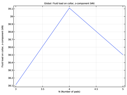
2
|
In the Settings window for 1D Plot Group, type Objective vs. Number of Pads in the Label text field.
|
|
3
|
Locate the Data section. From the Dataset list, choose Study 4: Shape Optimization Sweep/Parametric Solutions 1 (7) (sol5).
|
|
1
|
|
2
|
In the Settings window for Global, click Add Expression in the upper-right corner of the y-Axis Data section. From the menu, choose Component 1: Optimization (comp1) > Hydrodynamic Bearing > Fluid loads > Fluid load on collar (spatial and material frames) - N > hdb.htb1.Fcz - Fluid load on collar, z-component.
|
|
3
|
|
4
|
Locate the y-Axis Data section. In the table, enter the following settings:
|
|
5
|
|
6
|
|
1
|
|
2
|
|
3
|
|
4
|
|
5
|
|
1
|
|
2
|
|
1
|
|
2
|
|
3
|
|
1
|
|
2
|
|
3
|
Clear the Manual color range checkbox.
|
|
4
|
|
1
|
|
2
|
|
3
|
|
4
|
|
5
|
Select the Radius scale factor checkbox.
|
|
1
|
|
2
|
|
3
|
|
1
|
|
2
|
|
1
|
|
2
|