PDF

Minimizing the Flow Velocity in a Microchannel
Introduction
Topology optimization of the Navier–Stokes equations is encountered in different branches and applications, such as in the design of ventilation systems for cars and optimal reactors. A common technique applicable to such problems is to let the distribution of porous material vary continuously. In this model, the objective is to find the optimal distribution of a porous material in a microchannel such that the horizontal velocity component at the center of the channel is minimized.
The model is inspired by Ref. 1.
Model Definition
The model geometry (Figure 1) consists of three regions: the inlet channel, the design domain, and the outlet channel. A prescribed pressure drop between the inlet and the outlet drives the flow.
Figure 1: The model geometry.
The fluid flow in the channel is described by the Navier–Stokes equations
where −α(γ)u is a force term in which the coefficient
(1)
characterizes the flow in a porous medium. In Equation 1, α is interpreted as a continuous mapping determined by the function γ: Ω → [01], which in the limit of decreasing Darcy number and decreasing mesh size should be a discrete-valued function. When γ equals 1, α is zero, corresponding to free flow. Conversely, for γ = 0, α = αmax, where αmax is related to the dimensionless Darcy number, Da, according to
The convergence of the optimization process depends on three important factors: the Darcy number, the mesh size, and the coefficient q. Rewriting Equation 1 it is easily seen that α/αmax → 1 − γ in the limit q → ∞. In this limit, γ can be interpreted as the local porosity, ranging between 0 (filled) and 1 (open channel).
Results and Discussion
Figure 2 displays the design variable, γ, which represents the distribution of porous material. As the plot shows, γ is either 0 or 1 in most of the domain, with a narrow transition zone in between. The width of this transition zone is mesh dependent; you can reduce it by decreasing the mesh-element size. Alternatively, decreasing the Darcy number also gives harder boundaries at the interface between porous and open domains.
Figure 2: Distribution of porous material; the red areas represent open channel.
A question that naturally arises in this type of problems concerns uniqueness of the solution. In this case, there is at least one more solution that gives exactly the same result; because the channel has no upside or downside, a solution mirrored around the axis y = 0.5 mm would give exactly the same flow.
Figure 3 contains a surface plot of the horizontal velocity component and a streamline plot of the velocity field resulting from the optimization process. In addition, the contour γ = 0.5 indicates the border between the open channel and filling material. The plots reveal how the flow turns around, with a negative horizontal velocity at the center of the channel. Note also that the x-velocity has a minimum of roughly  14 mm/s at the design point.
Figure 3: The horizontal velocity (surface plot) and velocity field (streamlines) after optimization. In addition, the contour γ = 0.5 indicates the border between open channel and filling material.
If you were to increase the streamline density in the above plot, some streamlines passing through the barriers would appear. This effect is due to a small amount of leakage, which can be reduced further by increasing the mesh resolution.
Figure 4 shows the pressure distribution, verifying the prescribed pressure drop through the channel length. The pressure drop is naturally concentrated to the region with porous material.
Figure 4: Pressure distribution in the channel, the pressure drop is concentrated to the porous domain.
Reference
1. L. Højgaard Olesen, F. Okkels, and H. Bruus, “A High-level Programming-language Implementation of Topology Optimization Applied to Steady-state Navier–Stokes Flow,” Int. J. Numer. Methods Eng., vol. 65, pp. 975–1001, 2005.
Notes About the COMSOL Implementation
This model combines a Density Model feature with a Laminar Flow interface. First, you calculate the solution for the flow in an empty channel (that is, with no porous material). You then solve the optimization problem. In each iteration, the software calculates a solution for the flow problem and feeds it to the optimization routine, which updates the design variables.
If the specified convergence criterion is fulfilled, the solution process terminates; otherwise the new design-variable values are used in the next calculation of the flow problem. However, for design problems such as this one, there is a tradeoff between computation time and convergence. The solution may be sufficiently improved long before convergence is reached in the mathematical sense. Therefore, it is useful to limit the number of steps taken by the optimization algorithm after which the solution can be evaluated and restarted if not yet satisfactory.
Setting up this kind of model with a general optimization routine requires quite a bit of work, but as you will discover, solving this problem with the built-in tools for optimization in COMSOL Multiphysics is easy.
Application Library path: Optimization_Module/Topology_Optimization/reversed_flow
Modeling Instructions
From the File menu, choose New.
New
In the New window, click  Model Wizard.
Model Wizard
1
In the Model Wizard window, click  2D.
2
In the Select Physics tree, select Fluid Flow > Single-Phase Flow > Laminar Flow (spf).
3
Click Add.
4
Click  Study.
5
In the Select Study tree, select General Studies > Stationary.
6
Global Definitions
Parameters 1
1
In the Model Builder window, under Global Definitions click Parameters 1.
2
In the Settings window for Parameters, locate the Parameters section.
3
The purpose of the constant u0 is to introduce a rough velocity scale that you can use to make the objective function dimensionless with a value of the order 1.
Geometry 1
1
In the Model Builder window, under Component 1 (comp1) click Geometry 1.
2
In the Settings window for Geometry, locate the Units section.
3
From the Length unit list, choose mm.
Rectangle 1 (r1)
1
In the Geometry toolbar, click  Rectangle.
2
In the Settings window for Rectangle, locate the Size and Shape section.
3
In the Width text field, type 2.5.
Rectangle 2 (r2)
1
In the Geometry toolbar, click  Rectangle.
2
In the Settings window for Rectangle, locate the Size and Shape section.
3
In the Width text field, type 5.
4
Locate the Position section. In the x text field, type 2.5.
Rectangle 3 (r3)
1
In the Geometry toolbar, click  Rectangle.
2
In the Settings window for Rectangle, locate the Size and Shape section.
3
In the Width text field, type 2.5.
4
Locate the Position section. In the x text field, type 7.5.
Point 1 (pt1)
1
In the Geometry toolbar, click  Point.
2
In the Settings window for Point, locate the Point section.
3
In the x text field, type 5.
4
In the y text field, type 0.5.
5
Locate the Selections of Resulting Entities section. Select the Resulting objects selection checkbox.
6
Click  Build All Objects.
7
Click the  Zoom Extents button in the Graphics toolbar.
The geometry should now look like that in Figure 1.
Add Material
1
In the Materials toolbar, click  Add Material to open the Add Material window.
2
Go to the Add Material window.
3
In the tree, select Built-in > Water, liquid.
4
Click the Add to Component button in the window toolbar.
5
In the Materials toolbar, click  Add Material to close the Add Material window.
Materials
Water, liquid (mat1)
Next use the Density Model feature to set up the design variable.
Component 1 (comp1)
Density Model 1 (dtopo1)
1
In the Physics toolbar, click  Optimization and choose Topology Optimization.
Only the center part of the channel geometry is needed in the optimization, so you only have to define the control variable there.
2
3
In the Settings window for Density Model, locate the Filtering section.
4
From the Filter type list, choose None.
5
Locate the Interpolation section. From the Interpolation type list, choose Darcy.
6
In the q text field, type q.
7
Locate the Control Variable Initial Value section. In the θ0 text field, type 1.
This defines the shape functions for the design variable used in the optimization. The initial value 1 corresponds to a channel free from porous material.
Definitions
Variables 1
1
In the Definitions toolbar, click  Local Variables.
2
In the Settings window for Variables, locate the Geometric Entity Selection section.
3
From the Geometric entity level list, choose Domain.
4
The maximum damping is limited by the mesh size, because the mesh has to resolve the transition between marginal flow in the porous material and free flow in fluid region.
5
Locate the Variables section. In the table, enter the following settings:
Point Probe 1 (point1)
1
In the Definitions toolbar, click  Probes and choose Point Probe.
2
In the Settings window for Point Probe, type obj in the Variable name text field.
3
Locate the Source Selection section. From the Selection list, choose Point 1.
4
Click Replace Expression in the upper-right corner of the Expression section. From the menu, choose Component 1 (comp1) > Laminar Flow > Velocity and pressure > Velocity field - m/s > u - Velocity field, x-component.
This defines the objective function to be proportional to the x-component of the velocity at the center.
Laminar Flow (spf)
1
In the Model Builder window, under Component 1 (comp1) click Laminar Flow (spf).
2
In the Settings window for Laminar Flow, click to expand the Discretization section.
3
From the Discretization of fluids list, choose P2+P1.
This setting gives quadratic elements for the velocity field.
Volume Force 1
1
In the Physics toolbar, click  Domains and choose Volume Force.
In the next steps, you specify the pressure drop along the channel length by prescribing the pressure at the inlet and at the outlet. The resulting pressure gradient drives the flow in the channel.
2
3
In the Settings window for Volume Force, locate the Volume Force section.
4
Specify the F vector as
Inlet 1
1
In the Physics toolbar, click  Boundaries and choose Inlet.
2
3
In the Settings window for Inlet, locate the Boundary Condition section.
4
5
Locate the Pressure Conditions section. In the p0 text field, type 2.
Outlet 1
1
In the Physics toolbar, click  Boundaries and choose Outlet.
2
Keep all other boundaries at the default condition, which is the no-slip condition.
Mesh 1
This model is naturally highly dependent on the mesh size. In this example, choose a dense mesh; note, however, that this mesh can be further improved.
Free Triangular 1
In the Mesh toolbar, click  Free Triangular.
Size
1
In the Model Builder window, click Size.
2
In the Settings window for Size, locate the Element Size section.
3
Click the Custom button.
4
Locate the Element Size Parameters section. In the Maximum element growth rate text field, type 1.1.
Size 1
1
In the Model Builder window, right-click Free Triangular 1 and choose Size.
2
In the Settings window for Size, locate the Geometric Entity Selection section.
3
From the Geometric entity level list, choose Domain.
4
5
Locate the Element Size section. Click the Custom button.
6
Locate the Element Size Parameters section.
7
Select the Maximum element size checkbox. In the associated text field, type 0.08.
Size 2
1
Right-click Free Triangular 1 and choose Size.
2
In the Settings window for Size, locate the Geometric Entity Selection section.
3
From the Geometric entity level list, choose Point.
4
5
Locate the Element Size section. Click the Custom button.
6
Locate the Element Size Parameters section.
7
Select the Maximum element size checkbox. In the associated text field, type meshsz.
8
Click  Build All.
Although you can choose to solve the optimization problem directly, it can be good to check that the initial solution looks reasonable.
Study 1
In the Study toolbar, click  Compute.
Results
Probe Plot Group 1
The resulting plots show the magnitude of the velocity field, the pressure, and the design variable distribution in the channel. Proceed to solve the optimization problem.
Study 1
Topology Optimization
1
In the Study toolbar, click  Optimization and choose Topology Optimization.
2
In the Settings window for Topology Optimization, click Add Expression in the upper-right corner of the Objective Function section. From the menu, choose Component 1 (comp1) > Definitions > comp1.obj - Point Probe 1 - m/s.
3
Locate the Objective Function section. Find the Objective settings subsection. From the Objective scaling list, choose Initial solution based.
4
Click to expand the Output section. Select the Plot checkbox.
5
6
In the Study toolbar, click  Compute.
Results
Velocity (spf)
The default plot shows the magnitude of the velocity field in the channel. Generate Figure 3 with the following instructions:
Surface
1
In the Model Builder window, expand the Velocity (spf) node, then click Surface.
2
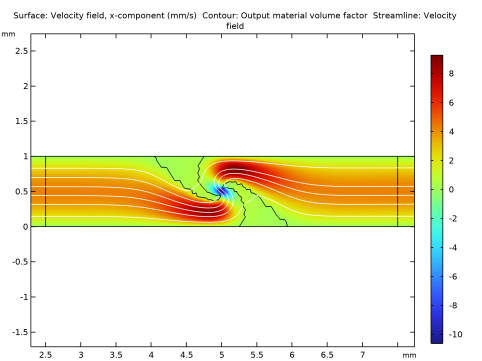
In the Settings window for Surface, click Replace Expression in the upper-right corner of the Expression section. From the menu, choose Component 1 (comp1) > Laminar Flow > Velocity and pressure > Velocity field - m/s > u - Velocity field, x-component.
3
Locate the Expression section. From the Unit list, choose mm/s.
Contour 1
1
In the Model Builder window, right-click Velocity (spf) and choose Contour.
2
In the Settings window for Contour, locate the Expression section.
3
In the Expression text field, type dtopo1.theta.
4
Locate the Levels section. From the Entry method list, choose Levels.
5
In the Levels text field, type 0.5.
6
Locate the Coloring and Style section. From the Coloring list, choose Uniform.
7
From the Color list, choose Black.
8
Clear the Color legend checkbox.
Streamline 1
1
Right-click Velocity (spf) and choose Streamline.
2
In the Settings window for Streamline, click Replace Expression in the upper-right corner of the Expression section. From the menu, choose Component 1 (comp1) > Laminar Flow > Velocity and pressure > u,v - Velocity field.
3
Locate the Streamline Positioning section. From the Positioning list, choose Magnitude controlled.
4
In the Minimum density level text field, type 0.
5
In the Maximum density level text field, type 10.9.
6
Locate the Coloring and Style section. Find the Point style subsection. From the Color list, choose White.
7
In the Velocity (spf) toolbar, click  Plot.
8
Click the Zoom Box button in the Graphics toolbar and then use the mouse to zoom in.
Pressure (spf)
The second default plot shows the pressure distribution Figure 4.
Output material volume factor
The last plot shows the material distribution in the channel Figure 2.
Objective Function History
1
In the Model Builder window, expand the Results > Topology Optimization node, then click Results > Probe Plot Group 1.
2
In the Settings window for 1D Plot Group, type Objective Function History in the Label text field.