
|


|
1
|
|
2
|
In the Select Physics tree, select Chemical Species Transport > Transport of Concentrated Species in Porous Media (tcs).
|
|
3
|
Click Add.
|
|
4
|
In the Select Physics tree, select Fluid Flow > Porous Media and Subsurface Flow > Darcy’s Law (dl).
|
|
5
|
Click Add.
|
|
6
|
In the Select Physics tree, select Heat Transfer > Porous Media > Heat Transfer in Porous Media (ht).
|
|
7
|
Click Add.
|
|
8
|
In the Select Physics tree, select Mathematics > ODE and DAE Interfaces > Domain ODEs and DAEs (dode).
|
|
9
|
Click Add.
|
|
10
|
In the Select Physics tree, select Mathematics > ODE and DAE Interfaces > Global ODEs and DAEs (ge).
|
|
11
|
Click Add.
|
|
12
|
Click
|
|
13
|
|
14
|
Click
|
|
1
|
|
2
|
|
3
|
|
4
|
Browse to the model’s Application Libraries folder and double-click the file pyrolysis_wood_odeobj_sample_properties_parameters.txt.
|
|
1
|
|
2
|
|
3
|
|
4
|
Browse to the model’s Application Libraries folder and double-click the file pyrolysis_wood_odeobj_experimental_conditions_parameters.txt.
|
|
1
|
|
2
|
|
3
|
|
4
|
Browse to the model’s Application Libraries folder and double-click the file pyrolysis_wood_odeobj_reaction_parameters.txt.
|
|
1
|
|
2
|
|
3
|
|
4
|
Browse to the model’s Application Libraries folder and double-click the file pyrolysis_wood_odeobj_parameters.txt.
|
|
1
|
In the Model Builder window, under Component 1 (comp1) right-click Definitions and choose Variables.
|
|
2
|
|
3
|
|
4
|
Browse to the model’s Application Libraries folder and double-click the file pyrolysis_wood_odeobj_solid_species_variables.txt.
|
|
1
|
|
2
|
|
3
|
|
4
|
Browse to the model’s Application Libraries folder and double-click the file pyrolysis_wood_odeobj_reaction_variables.txt.
|
|
1
|
|
2
|
|
3
|
|
4
|
Browse to the model’s Application Libraries folder and double-click the file pyrolysis_wood_odeobj_fluid_species_variables.txt.
|
|
1
|
|
2
|
|
3
|
|
4
|
Browse to the model’s Application Libraries folder and double-click the file pyrolysis_wood_odeobj_surface_variables.txt.
|
|
1
|
|
2
|
|
3
|
|
4
|
|
1
|
|
2
|
|
3
|
|
4
|
Click
|
|
5
|
|
1
|
|
2
|
|
3
|
|
4
|
Click
|
|
1
|
|
2
|
On the object fin, select Boundary 7 only.
|
|
3
|
|
1
|
|
2
|
|
3
|
Click
|
|
4
|
|
5
|
|
6
|
Click OK.
|
|
7
|
|
8
|
In the Source term quantity table, enter the following settings:
|
|
9
|
|
10
|
|
11
|
In the Dependent variables (kg/m³) table, enter the following settings:
|
|
1
|
In the Model Builder window, under Component 1 (comp1) > Domain ODEs and DAEs (dode) click Distributed ODE 1.
|
|
2
|
|
3
|
|
4
|
|
5
|
In the f text-field array, type k_c*rho_is+k_c2*tcs.rho*w_t on the third row. The dependent variable w_t is not yet defined. It will be added in the Transport of Concentrated Species in Porous Media Interface.
|
|
1
|
|
2
|
|
3
|
|
1
|
In the Model Builder window, under Component 1 (comp1) click Transport of Concentrated Species in Porous Media (tcs).
|
|
2
|
In the Settings window for Transport of Concentrated Species in Porous Media, locate the Transport Mechanisms section.
|
|
3
|
|
4
|
|
5
|
In the Mass fractions (1) table, enter the following settings:
|
|
6
|
|
1
|
In the Model Builder window, under Component 1 (comp1) > Transport of Concentrated Species in Porous Media (tcs) click Species Molar Masses 1.
|
|
2
|
|
3
|
|
4
|
|
5
|
In the MwN2 text field, type Mw_N2. The parameters for the molar masses were loaded from file and can be found in the Sample Properties node under Global Definitions.
|
|
1
|
In the Model Builder window, under Component 1 (comp1) > Transport of Concentrated Species in Porous Media (tcs) > Porous Medium 1 click Fluid 1.
|
|
2
|
|
3
|
|
1
|
|
2
|
|
3
|
|
1
|
In the Model Builder window, under Component 1 (comp1) > Transport of Concentrated Species in Porous Media (tcs) click Initial Values 1.
|
|
2
|
|
3
|
|
4
|
|
1
|
|
1
|
|
2
|
In the Settings window for Reaction Sources, type Reaction Sources with Phase Transfer in the Label text field.
|
|
4
|
|
5
|
|
6
|
|
1
|
|
2
|
In the Settings window for Reaction Sources, type Reaction Sources Gas to Gas in the Label text field.
|
|
4
|
|
5
|
|
1
|
In the Model Builder window, under Component 1 (comp1) > Darcy’s Law (dl) > Porous Medium 1 click Fluid 1.
|
|
2
|
|
3
|
|
4
|
|
1
|
|
2
|
|
3
|
|
4
|
|
5
|
Specify the κ matrix as
|
|
1
|
|
3
|
|
4
|
Click in the Qm text field, then press Ctrl+Space. From the menu, choose Component 1 (comp1) > Transport of Concentrated Species in Porous Media > tcs.Qmass - Net mass source - kg/(m³·s).
|
|
1
|
|
1
|
|
1
|
In the Model Builder window, under Component 1 (comp1) > Heat Transfer in Porous Media (ht) > Porous Medium 1 click Fluid 1.
|
|
2
|
|
3
|
|
4
|
|
5
|
Locate the Heat Conduction, Fluid section. From the kf list, choose User defined. In the associated text field, type k_f.
|
|
6
|
|
7
|
|
1
|
|
2
|
|
3
|
|
4
|
Locate the Heat Conduction, Porous Matrix section. From the kb list, choose User defined. From the list, choose Diagonal.
|
|
5
|
|
6
|
Locate the Thermodynamics, Porous Matrix section. From the ρb list, choose User defined. In the associated text field, type rho_b.
|
|
7
|
|
1
|
In the Model Builder window, under Component 1 (comp1) > Heat Transfer in Porous Media (ht) click Initial Values 1.
|
|
2
|
|
3
|
|
1
|
|
1
|
|
3
|
|
4
|
|
1
|
|
3
|
|
4
|
|
1
|
|
2
|
|
3
|
From the list, choose User-controlled mesh.
|
|
1
|
|
2
|
|
3
|
|
1
|
|
2
|
Drag and drop below Size.
|
|
3
|
|
4
|
|
1
|
|
3
|
|
4
|
|
5
|
|
1
|
|
3
|
|
4
|
|
1
|
|
2
|
|
3
|
|
5
|
|
6
|
|
1
|
|
2
|
In the Settings window for Study, type Study 1: Forward Model (Initial-Value Based) in the Label text field.
|
|
3
|
|
1
|
In the Model Builder window, under Study 1: Forward Model (Initial-Value Based) click Step 1: Time Dependent.
|
|
2
|
|
3
|
|
4
|
|
5
|
Locate the Physics and Variables Selection section. In the Solve for column of the table, under Component 1 (comp1), clear the checkbox for Global ODEs and DAEs (ge).
|
|
1
|
|
2
|
In the Model Builder window, expand the Solution 1 (sol1) node. The choice Show Default Solver creates the node Solver Configurations where we can edit the solver settings. Since we know the scales for the dependent variables, we will enter them and not use the default values. If a scale is too high (orders higher than the value of the dependent variable), then we will not get an accurate solution for that variable. If instead the scales are too low, the solver will take more time steps than necessary, giving high accuracy but increasing the computation time.
|
|
3
|
In the Model Builder window, expand the Study 1: Forward Model (Initial-Value Based) > Solver Configurations > Solution 1 (sol1) > Dependent Variables 1 node, then click Pressure (comp1.p).
|
|
4
|
|
5
|
|
6
|
In the Model Builder window, under Study 1: Forward Model (Initial-Value Based) > Solver Configurations > Solution 1 (sol1) > Dependent Variables 1 click Dependent Variable Rho_c (comp1.rho_c).
|
|
7
|
|
8
|
|
9
|
|
10
|
In the Model Builder window, under Study 1: Forward Model (Initial-Value Based) > Solver Configurations > Solution 1 (sol1) > Dependent Variables 1 click Dependent Variable Rho_is (comp1.rho_is).
|
|
11
|
|
12
|
|
13
|
|
14
|
In the Model Builder window, under Study 1: Forward Model (Initial-Value Based) > Solver Configurations > Solution 1 (sol1) > Dependent Variables 1 click Dependent Variable Rho_w (comp1.rho_w).
|
|
15
|
|
16
|
|
17
|
In the Model Builder window, under Study 1: Forward Model (Initial-Value Based) > Solver Configurations > Solution 1 (sol1) > Dependent Variables 1 click Temperature (comp1.T).
|
|
18
|
|
19
|
|
20
|
In the Model Builder window, under Study 1: Forward Model (Initial-Value Based) > Solver Configurations > Solution 1 (sol1) > Dependent Variables 1 click Mass Fraction (comp1.w_g).
|
|
21
|
|
22
|
|
23
|
|
24
|
In the Model Builder window, under Study 1: Forward Model (Initial-Value Based) > Solver Configurations > Solution 1 (sol1) > Dependent Variables 1 click Mass Fraction (comp1.w_t).
|
|
25
|
|
26
|
|
27
|
|
1
|
|
2
|
|
3
|
|
1
|
|
2
|
|
3
|
Click
|
|
4
|
Browse to the model’s Application Libraries folder and double-click the file pyrolysis_wood_odeobj_experimental_data_Y.txt.
|
|
5
|
|
6
|
Locate the Column Headers section. In the table, enter the following settings:
|
|
1
|
|
2
|
|
3
|
|
4
|
Browse to the model’s Application Libraries folder and double-click the file pyrolysis_wood_odeobj_experimental_data_T_surface.txt.
|
|
5
|
Locate the Column Headers section. In the table, enter the following settings:
|
|
1
|
|
2
|
|
3
|
|
4
|
Browse to the model’s Application Libraries folder and double-click the file pyrolysis_wood_odeobj_experimental_data_T_middle.txt.
|
|
5
|
Locate the Column Headers section. In the table, enter the following settings:
|
|
1
|
|
2
|
|
3
|
|
4
|
Browse to the model’s Application Libraries folder and double-click the file pyrolysis_wood_odeobj_experimental_data_T_center.txt.
|
|
5
|
Locate the Column Headers section. In the table, enter the following settings:
|
|
1
|
|
2
|
|
3
|
|
4
|
|
1
|
|
2
|
|
3
|
|
4
|
|
5
|
|
6
|
|
7
|
|
8
|
Clear the Headers checkbox.
|
|
9
|
|
1
|
|
2
|
|
3
|
|
4
|
|
5
|
|
1
|
|
2
|
|
3
|
|
4
|
|
5
|
|
1
|
|
2
|
|
3
|
|
4
|
|
5
|
|
1
|
|
2
|
|
3
|
Select the Two y-axes checkbox.
|
|
4
|
|
5
|
|
6
|
|
7
|
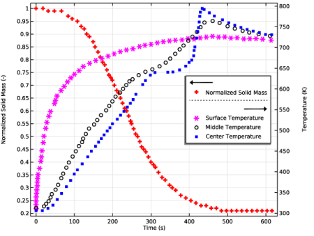
In the table, select the Plot on secondary y-axis checkboxes for Surface Temperature, Middle Temperature, and Center Temperature.
|
|
8
|
|
9
|
|
10
|
|
1
|
In the Model Builder window, under Component 1 (comp1) right-click Definitions and choose Node Group.
|
|
2
|
|
1
|
|
2
|
|
3
|
|
5
|
|
6
|
Select the Description checkbox.
|
|
1
|
|
2
|
|
3
|
|
1
|
|
2
|
|
3
|
|
1
|
|
2
|
|
3
|
|
4
|
|
5
|
Select the Description checkbox.
|
|
1
|
|
1
|
|
2
|
|
3
|
|
4
|
Select the Keep child nodes checkbox.
|
|
5
|
|
6
|
|
1
|
|
2
|
In the Settings window for Surface Integration, type Gas and Tar Inside Sample in the Label text field.
|
|
4
|
|
1
|
In the Model Builder window, right-click Mass Conservation Check and choose Integration > Line Integration.
|
|
2
|
In the Settings window for Line Integration, type Gas and Tar Leaving Sample in the Label text field.
|
|
3
|
|
6
|
|
7
|
Select the Cumulative checkbox.
|
|
1
|
|
3
|
|
4
|
|
1
|
|
2
|
|
3
|
|
1
|
|
2
|
|
3
|
|
4
|
|
1
|
Go to the Mass Conservation Check window.
|
|
2
|
|
3
|
|
4
|
|
5
|
Go to the Mass Conservation Check window.
|
|
1
|
|
2
|
|
3
|
|
4
|
Locate the Data Column Settings section. In the table, click to select the cell at row number 1 and column number 3.
|
|
5
|
|
1
|
|
2
|
|
3
|
|
4
|
|
1
|
|
2
|
|
3
|
|
1
|
|
2
|
|
3
|
|
1
|
In the Model Builder window, under Component 1 (comp1) right-click Definitions and choose Variables.
|
|
2
|
|
3
|
Locate the Variables section. In the table, enter the following settings:
|
|
1
|
In the Model Builder window, under Component 1 (comp1) > Global ODEs and DAEs (ge) click Global Equations 1 (ODE1).
|
|
2
|
|
1
|
|
2
|
Go to the Add Study window.
|
|
3
|
|
4
|
Click the Add Study button in the window toolbar.
|
|
5
|
|
1
|
|
2
|
|
1
|
|
2
|
|
3
|
|
4
|
|
5
|
Click Add Expression in the upper-right corner of the Objective Function section. From the menu, choose Component 1 (comp1) > Global ODEs and DAEs > comp1.obj - State variable obj - 1.
|
|
6
|
|
8
|
Click to expand the Solver Settings section. Find the Objective settings subsection. From the Objective scaling list, choose Initial solution based.
|
|
9
|
|
1
|
|
2
|
|
3
|
|
1
|
|
2
|
|
3
|
In the Model Builder window, expand the Study 2: Parameter Estimation > Solver Configurations > Solution 2 (sol2) > Dependent Variables 1 node, then click Pressure (comp1.p).
|
|
4
|
|
5
|
|
6
|
In the Model Builder window, under Study 2: Parameter Estimation > Solver Configurations > Solution 2 (sol2) > Dependent Variables 1 click Dependent Variable Rho_c (comp1.rho_c).
|
|
7
|
|
8
|
|
9
|
|
10
|
In the Model Builder window, under Study 2: Parameter Estimation > Solver Configurations > Solution 2 (sol2) > Dependent Variables 1 click Dependent Variable Rho_is (comp1.rho_is).
|
|
11
|
|
12
|
|
13
|
|
14
|
In the Model Builder window, under Study 2: Parameter Estimation > Solver Configurations > Solution 2 (sol2) > Dependent Variables 1 click Dependent Variable Rho_w (comp1.rho_w).
|
|
15
|
|
16
|
|
17
|
In the Model Builder window, under Study 2: Parameter Estimation > Solver Configurations > Solution 2 (sol2) > Dependent Variables 1 click Temperature (comp1.T).
|
|
18
|
|
19
|
|
20
|
In the Model Builder window, under Study 2: Parameter Estimation > Solver Configurations > Solution 2 (sol2) > Dependent Variables 1 click Mass Fraction (comp1.w_g).
|
|
21
|
|
22
|
|
23
|
|
24
|
In the Model Builder window, under Study 2: Parameter Estimation > Solver Configurations > Solution 2 (sol2) > Dependent Variables 1 click Mass Fraction (comp1.w_t).
|
|
25
|
|
26
|
|
27
|
|
28
|
In the Model Builder window, expand the Study 2: Parameter Estimation > Solver Configurations > Solution 2 (sol2) > Optimization Solver 1 node, then click Time-Dependent Solver 1.
|
|
29
|
|
30
|
|
31
|
In the Model Builder window, expand the Study 2: Parameter Estimation > Solver Configurations > Solution 2 (sol2) > Optimization Solver 1 > Time-Dependent Solver 1 node, then click Advanced.
|
|
32
|
|
33
|
|
34
|
In the Model Builder window, under Study 2: Parameter Estimation > Solver Configurations > Solution 2 (sol2) > Optimization Solver 1 > Time-Dependent Solver 1 click Direct, pressure (dl) (Merged).
|
|
35
|
|
36
|
|
1
|
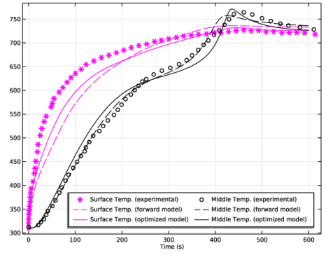
In the Settings window for 1D Plot Group, type Optimized, Forward Model, and Experimental Data: T_surface and T_middle in the Label text field.
|
|
2
|
In the Model Builder window, expand the Optimized, Forward Model, and Experimental Data: T_surface and T_middle node.
|
|
1
|
In the Model Builder window, under Results > Optimized, Forward Model, and Experimental Data: T_surface and T_middle, Ctrl-click to select Normalized Solid Mass and Center Temperature.
|
|
2
|
Right-click and choose Delete.
|
|
1
|
In the Model Builder window, under Results > Optimized, Forward Model, and Experimental Data: T_surface and T_middle click Middle Temperature.
|
|
2
|
|
1
|
In the Model Builder window, right-click Optimized, Forward Model, and Experimental Data: T_surface and T_middle and choose Point Graph.
|
|
3
|
|
4
|
Locate the Data section. From the Dataset list, choose Study 1: Forward Model (Initial-Value Based)/Solution 1 (sol1).
|
|
6
|
|
7
|
Click to expand the Coloring and Style section. Find the Line style subsection. From the Line list, choose Dashed.
|
|
8
|
|
9
|
|
10
|
|
11
|
Clear the Point checkbox.
|
|
12
|
Clear the Solution checkbox.
|
|
1
|
|
2
|
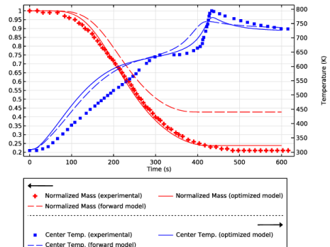
In the Settings window for Point Graph, type Surface Temp. (optimized model) in the Label text field.
|
|
3
|
Locate the Data section. From the Dataset list, choose Study 2: Parameter Estimation/Solution 2 (sol2).
|
|
4
|
Locate the Coloring and Style section. Find the Line style subsection. From the Line list, choose Solid.
|
|
1
|
|
2
|
|
3
|
|
5
|
|
1
|
|
2
|
|
3
|
|
4
|
|
5
|
Locate the Coloring and Style section. Find the Line style subsection. From the Line list, choose Solid.
|
|
1
|
In the Model Builder window, click Optimized, Forward Model, and Experimental Data: T_surface and T_middle.
|
|
2
|
|
3
|
Clear the Two y-axes checkbox.
|
|
4
|
|
5
|
|
6
|
|
7
|
|
8
|
|
1
|
|
2
|
Drag and drop below Surface Temp. (optimized model).
|
|
1
|
In the Model Builder window, under Results > Experimental Data 2, Ctrl-click to select Surface Temperature and Middle Temperature.
|
|
2
|
Right-click and choose Delete.
|
|
1
|
|
2
|
In the Settings window for 1D Plot Group, type Optimized, Forward Model, and Experimental Data: Y and T_center in the Label text field.
|
|
3
|
|
4
|
|
5
|
|
1
|
In the Model Builder window, under Results > Optimized, Forward Model, and Experimental Data: Y and T_center click Normalized Solid Mass.
|
|
2
|
In the Settings window for Table Graph, type Normalized Mass (experimental) in the Label text field.
|
|
1
|
In the Model Builder window, under Results > Optimized, Forward Model, and Experimental Data: Y and T_center click Center Temperature.
|
|
2
|
|
1
|
|
2
|
Locate the Data section. From the Dataset list, choose Study 1: Forward Model (Initial-Value Based)/Solution 1 (sol1).
|
|
3
|
Click Replace Expression in the upper-right corner of the y-Axis Data section. From the menu, choose Component 1 (comp1) > Definitions > domY - Domain Probe Y - 1.
|
|
4
|
Click to expand the Coloring and Style section. Find the Line style subsection. From the Line list, choose Dashed.
|
|
5
|
|
6
|
|
7
|
Clear the Solution checkbox.
|
|
8
|
Clear the Description checkbox.
|
|
1
|
|
2
|
|
3
|
Locate the Data section. From the Dataset list, choose Study 2: Parameter Estimation/Solution 2 (sol2).
|
|
4
|
Locate the Coloring and Style section. Find the Line style subsection. From the Line list, choose Solid.
|
|
1
|
In the Model Builder window, right-click Optimized, Forward Model, and Experimental Data: Y and T_center and choose Point Graph.
|
|
2
|
|
3
|
Locate the Data section. From the Dataset list, choose Study 1: Forward Model (Initial-Value Based)/Solution 1 (sol1).
|
|
4
|
|
5
|
|
6
|
Locate the Coloring and Style section. Find the Line style subsection. From the Line list, choose Dashed.
|
|
7
|
|
8
|
|
9
|
|
10
|
Clear the Point checkbox.
|
|
11
|
Clear the Solution checkbox.
|
|
1
|
|
2
|
In the Settings window for Point Graph, type Center Temp. (optimized model) in the Label text field.
|
|
3
|
Locate the Data section. From the Dataset list, choose Study 2: Parameter Estimation/Solution 2 (sol2).
|
|
4
|
Locate the Coloring and Style section. Find the Line style subsection. From the Line list, choose Solid.
|
|
5
|
|
1
|
|
2
|
|
3
|
Select the Plot checkbox.
|
|
5
|
|
1
|
In the Model Builder window, under Results click Optimized, Forward Model, and Experimental Data: T_surface and T_middle.
|
|
2
|
|
3
|
|
1
|
|
2
|
|
3
|
|
1
|
|
2
|
In the Settings window for Evaluation Group, type Optimized parameter values in the Label text field.
|
|
3
|
Locate the Data section. From the Dataset list, choose Study 2: Parameter Estimation/Solution 2 (sol2).
|
|
4
|
|
1
|
|
2
|
In the Settings window for Global Evaluation, click Add Expression in the upper-right corner of the Expressions section. From the menu, choose Global definitions > Parameters > A_is - Frequency factor w -> is (intermediate solid) - 1/s.
|
|
3
|
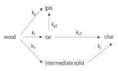
Click Add Expression in the upper-right corner of the Expressions section. From the menu, choose Global definitions > Parameters > DH_c - Heat of reaction intermediate solid -> char - J/kg.
|
|
4
|
Click Add Expression in the upper-right corner of the Expressions section. From the menu, choose Global definitions > Parameters > DH_t - Heat of reaction wood -> tar - J/kg.
|
|
5
|
Click Add Expression in the upper-right corner of the Expressions section. From the menu, choose Global definitions > Parameters > hconv - External convective heat transfer coefficient - W/(m²·K).
|
|
6
|
|
1
|
|
2
|
|
3
|
Locate the Data section. From the Dataset list, choose Study 2: Parameter Estimation/Solution 2 (sol2).
|
|
1
|
|
2
|
|
4
|
|
5
|
|
1
|
|
2
|
|
3
|
|
4
|
|
5
|
|
6
|
|
1
|
|
2
|
|
3
|
|
4
|
|
5
|
Click
|
|
1
|
|
2
|
|
3
|
|
4
|
|
5
|
Click
|
|
1
|
|
2
|
|
3
|
|
4
|
|
5
|
|
6
|
|
7
|
|
8
|
|
9
|
|
10
|
Click OK.
|
|
1
|
|
2
|
|
3
|
Locate the Definition section. In the table, enter the following settings:
|
|
1
|
|
2
|
|
3
|
Locate the Definition section. In the table, enter the following settings:
|
|
1
|
|
2
|
|
3
|
Locate the Definition section. In the table, enter the following settings:
|
|
1
|
|
2
|
|
3
|
|
4
|
|
5
|
|
1
|
|
2
|
|
3
|
|
4
|
|
1
|
|
2
|
|
3
|
|
4
|
|
5
|
|
6
|
|
1
|
|
2
|
|
3
|
|
4
|
|
5
|
|
6
|
|
1
|
|
2
|
|
3
|
|
4
|
|
5
|
|
6
|
|
7
|
|
1
|
|
2
|
|
3
|
|
4
|
|
5
|
|
1
|
|
2
|
|
3
|
|
4
|
|
1
|
|
2
|
|
3
|
|
4
|
|
1
|
|
2
|
|
3
|
|
4
|
|
1
|
|
2
|
|
3
|
|
1
|
|
2
|
|
3
|
|
4
|
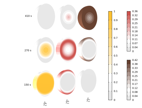
Locate the Annotation section. In the Text text field, type $\frac{\rho_{\omega}}{\rho_{\omega,0}}$.
|
|
5
|
Select the LaTeX markup checkbox.
|
|
6
|
|
7
|
|
8
|
|
9
|
|
1
|
|
2
|
|
3
|
|
4
|
|
1
|
|
2
|
|
3
|
|
4
|
|
1
|
|
2
|
|
3
|
|
4
|
|
5
|
|
1
|
|
2
|
|
3
|
|
4
|
|
1
|
|
2
|
|
3
|
|
4
|
|
1
|
|
2
|
|
3
|
|
4
|
|
5
|
|
1
|
|
2
|
|
3
|
|
4
|
|
5
|
|
6
|
|
7
|
|
8
|
|
9
|
|
10
|
|
11
|
|
1
|
|
2
|
|
3
|
|
4
|
Select the LaTeX markup checkbox.
|
|
5
|
|
6
|
|
7
|
|
8
|
|
9
|
|
1
|
|
2
|
|
3
|
|
4
|
|
1
|
|
2
|
|
3
|
|
4
|
|
1
|
|
2
|
|
3
|
|
4
|
|
5
|
|
1
|
|
2
|
|
3
|
|
4
|
|
5
|
|
6
|
|
1
|
|
2
|
|
3
|
|
4
|
|
5
|
|
1
|
|
2
|
|
3
|
|
4
|
|
5
|
|
1
|
|
2
|
|
3
|
|
4
|
|
5
|
|
6
|
|
1
|
|
2
|
|
3
|
|
4
|
|
5
|
|
1
|
|
2
|
In the Settings window for 2D Plot Group, type Pressure, velocity, porosity, and normalized solid mass at 270 s in the Label text field.
|
|
3
|
|
4
|
|
5
|
|
6
|
|
7
|
|
8
|
|
9
|
|
10
|
|
1
|
|
2
|
|
3
|
|
4
|
Select the LaTeX markup checkbox.
|
|
5
|
|
6
|
|
7
|
|
8
|
|
9
|
|
1
|
|
2
|
|
3
|
|
4
|
|
1
|
|
2
|
|
3
|
|
4
|
|
5
|
|
1
|
|
2
|
|
3
|
|
4
|
|
1
|
In the Model Builder window, right-click Pressure, velocity, porosity, and normalized solid mass at 270 s and choose Surface.
|
|
2
|
|
3
|
|
4
|
|
5
|
|
1
|
|
2
|
|
3
|
|
4
|
|
5
|
|
1
|
In the Model Builder window, right-click Pressure, velocity, porosity, and normalized solid mass at 270 s and choose Arrow Surface.
|
|
2
|
|
3
|
|
4
|
|
5
|
Locate the Arrow Positioning section. Find the R grid points subsection. In the Points text field, type 10.
|
|
6
|
|
7
|
|
8
|
|
9
|
|
10
|
|
11
|
|
12
|
|
13
|
|
1
|
|
2
|
|
3
|
|
4
|
|
5
|
|
6
|
|
1
|
|
2
|
|
3
|
|
4
|
|
5
|
|
6
|
|
1
|
|
2
|
In the Model Builder window, click Pressure, velocity, porosity, and normalized solid mass at 270 s.
|
|
3
|