PDF

Time-Optimal Control for Heating of a Rod
Introduction
Time-optimal control is a type of optimization specific to transient problems. Typically, a number of scalar parameters are allowed to vary in time within certain bounds, and one then has to find the optimal transient variation of these parameters with respect to some objective and, possibly, constraints. This model demonstrates optimal control for a simple heating example using the Control Function feature.
Model Definition
The model geometry consists of a rod that is 3 m long and 1 cm in diameter. The rod is made of structural steel and the idea is to heat it as fast as possible without exceeding a specified maximum temperature. Once a certain target temperature is reached, the process is complete, and the objective is to minimize the processing time. The simple geometry of the problem means that the minimum temperature occurs in the center, while the maximum occurs on the boundary. If unlimited power is available, one can thus solve the problem by applying the maximum temperature on the boundary and computing the power as a results-processing step. When the available power is limited, one has to apply the maximum power and switch to temperature control when the maximum temperature is reached on the boundary.
This example uses a Control Function feature for the power and minimizes the processing time with constraints on the inner temperature at the final time and the outer temperature for all times.
The model uses 260°C as the target temperature, 20°C as the initial temperature, and 270°C as the maximum temperature. The maximum heating power is 200 kW.
The processing time is defined as a parameter so that it can be used in the argument for the Control Function feature, which ensures that the entire range of the function is used.
Results and Discussion
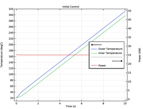
Figure 1 displays the temperature on the inside and the outside of the rod for the initial uniform heating. The temperatures increase linearly with time, resulting in excessive heating.
Figure 1: The initial temperature at the surface of the cylinder for a heating power corresponding to 50% of the maximum power. The temperature for the optimized solution is also shown. The control function values are plotted on the second y-axis.
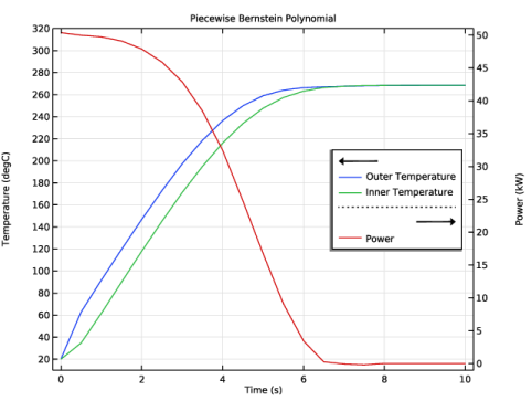
Figure 2: The temperature and heating as functions of time for the case of a control function regularized via a piecewise Bernstein polynomial. The heating is plotted on the second y-axis.
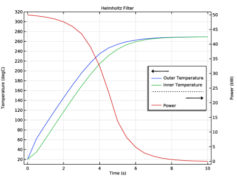
Figure 2 shows the result of optimization with a piecewise function consisting of three 3rd order Bernstein polynomials, while Figure 3 shows the case of a Helmholtz filter with a maximum slope 10 times the slope corresponding to a steady increase from the minimum to the maximum. The resulting controls and temperature are similar, and excessive heating is avoided in both cases.
Figure 3: The temperature and heating as functions of time for the case of a control function regularized via Helmholtz filtering. The heating is plotted on the second y-axis.
Application Library path: Optimization_Module/Optimal_Control/optimal_heating_control
Modeling Instructions
From the File menu, choose New.
New
In the New window, click  Model Wizard.
Model Wizard
1
In the Model Wizard window, click  1D Axisymmetric.
2
In the Select Physics tree, select Heat Transfer > Heat Transfer in Solids (ht).
3
Click Add.
4
In the Select Physics tree, select Mathematics > ODE and DAE Interfaces > Global ODEs and DAEs (ge).
5
Click Add.
6
Click  Study.
7
In the Select Study tree, select General Studies > Time Dependent.
8
Global Definitions
Parameters 1
1
In the Model Builder window, under Global Definitions click Parameters 1.
2
In the Settings window for Parameters, locate the Parameters section.
3
Geometry 1
Interval 1 (i1)
1
In the Model Builder window, under Component 1 (comp1) right-click Geometry 1 and choose Interval.
2
In the Settings window for Interval, locate the Interval section.
3
Definitions
Outer Temperature
1
In the Definitions toolbar, click  Probes and choose Point Probe.
2
In the Settings window for Point Probe, type Outer Temperature in the Label text field.
3
In the Variable name text field, type Tout.
4
Inner Temperature
1
Right-click Outer Temperature and choose Duplicate.
2
In the Settings window for Point Probe, type Inner Temperature in the Label text field.
3
In the Variable name text field, type Tin.
4
Temperature Error
1
In the Definitions toolbar, click  Probes and choose Global Variable Probe.
2
In the Settings window for Global Variable Probe, type Temperature Error in the Label text field.
3
In the Variable name text field, type Terror.
4
Locate the Expression section. In the Expression text field, type (1-(Tout-T0)/(Ttarget-T0))^2.
Add Material
1
In the Materials toolbar, click  Add Material to open the Add Material window.
2
Go to the Add Material window.
3
In the tree, select Built-in > Structural steel.
4
Click the Add to Component button in the window toolbar.
5
In the Materials toolbar, click  Add Material to close the Add Material window.
Heat Transfer in Solids (ht)
Initial Values 1
1
In the Settings window for Initial Values, locate the Initial Values section.
2
In the T text field, type T0.
Definitions (comp1)
Control Function (Piecewise Polynomial)
1
In the Definitions toolbar, click  Control Variables and choose Control Function.
2
In the Settings window for Control Function, type Control Function (Piecewise Polynomial) in the Label text field.
3
Locate the Input section. In the xend text field, type tmax.
4
Locate the Control Variable Discretization section. From the Control type list, choose Piecewise Bernstein polynomial.
5
In the Order text field, type 3.
6
In the Number of segments text field, type 3.
Control Function (Helmholtz)
1
Right-click Control Function (Piecewise Polynomial) and choose Duplicate.
2
In the Settings window for Control Function, type Control Function (Helmholtz) in the Label text field.
3
Locate the Control Variable Discretization section. From the Control type list, choose Helmholtz filter.
4
In the fmax text field, type 10/tmax.
Heat Transfer in Solids (ht)
1
In the Model Builder window, under Component 1 (comp1) click Heat Transfer in Solids (ht).
2
In the Settings window for Heat Transfer in Solids, locate the Physical Model section.
3
In the dz text field, type Lz.
Heat Flux 1
1
In the Physics toolbar, click  Boundaries and choose Heat Flux.
2
3
In the Settings window for Heat Flux, locate the Heat Flux section.
4
From the Flux type list, choose Heat rate.
5
In the P0 text field, type cfunc1(t)*Pmax.
Heat Flux 2
1
Right-click Heat Flux 1 and choose Duplicate.
2
In the Settings window for Heat Flux, locate the Heat Flux section.
3
In the P0 text field, type cfunc2(t)*Pmax.
Global ODEs and DAEs (ge)
Global Equations 1 (ODE1)
Use the ODE to integrate the squared error over time.
1
In the Model Builder window, under Component 1 (comp1) > Global ODEs and DAEs (ge) click Global Equations 1 (ODE1).
2
In the Settings window for Global Equations, locate the Global Equations section.
3
Mesh 1
Edge 1
In the Mesh toolbar, click  Edge.
Size
1
In the Model Builder window, click Size.
2
In the Settings window for Size, locate the Element Size section.
3
From the Predefined list, choose Extra fine.
4
Click  Build All.
Study 1: Initial Control
1
In the Model Builder window, click Study 1.
2
In the Settings window for Study, type Study 1: Initial Control in the Label text field.
Step 1: Time Dependent
1
In the Model Builder window, under Study 1: Initial Control click Step 1: Time Dependent.
2
In the Settings window for Time Dependent, locate the Study Settings section.
3
In the Output times text field, type range(0,tmax/20,tmax).
4
Click to expand the Results While Solving section. From the Probes list, choose None.
5
Locate the Physics and Variables Selection section. Select the Modify model configuration for study step checkbox.
6
In the tree, select Component 1 (comp1) > Heat Transfer in Solids (ht) > Heat Flux 2.
7
Click  Disable.
8
In the Study toolbar, click  Compute.
Results
Line Graph 1
1
In the Model Builder window, expand the Temperature (ht) node.
2
Right-click Line Graph 1 and choose Delete.
Global 1
1
Right-click Temperature (ht) and choose Global.
2
In the Settings window for Global, click Replace Expression in the upper-right corner of the y-Axis Data section. From the menu, choose Component 1 (comp1) > Definitions > Tout - Outer Temperature - K.
3
Click Replace Expression in the upper-right corner of the y-Axis Data section. From the menu, choose Component 1 (comp1) > Definitions > Tin - Inner Temperature - K.
4
Locate the y-Axis Data section. In the table, enter the following settings:
5
Click to expand the Legends section.
Global 2
1
Right-click Global 1 and choose Duplicate.
2
In the Settings window for Global, locate the y-Axis Data section.
3
Click  Clear Table.
4
Click Add Expression in the upper-right corner of the y-Axis Data section. From the menu, choose Component 1 (comp1) > Heat Transfer in Solids > Heat and energy balance > Energy balance > Net powers, boundary features > ht.hf1.ntefluxInt - Total net energy rate - W.
5
Locate the y-Axis Data section. In the table, enter the following settings:
Initial Control
1
In the Model Builder window, under Results click Temperature (ht).
2
In the Settings window for 1D Plot Group, type Initial Control in the Label text field.
3
Click to expand the Title section. From the Title type list, choose Label.
4
Locate the Plot Settings section.
5
Select the y-axis label checkbox. In the associated text field, type Temperature (degC).
6
Select the Two y-axes checkbox.
7
In the table, select the Plot on secondary y-axis checkbox for Global 2.
8
Select the Secondary y-axis label checkbox. In the associated text field, type Power (kW).
9
Locate the Axis section. Select the Manual axis limits checkbox.
10
In the x minimum text field, type -tmax/50.
11
In the x maximum text field, type tmax*1.02.
12
In the y minimum text field, type 10.
13
In the y maximum text field, type 320.
14
In the Secondary y minimum text field, type -Pmax*2e-5.
15
In the Secondary y maximum text field, type Pmax*1.02e-3.
16
Locate the Legend section. From the Position list, choose Middle right.
17
In the Initial Control toolbar, click  Plot.
1D Plot Group 2
In the Model Builder window, right-click 1D Plot Group 2 and choose Delete.
Add Study
In the Home toolbar, click  Add Study to open the Add Study window.
Add Study
1
Go to the Add Study window.
2
Find the Studies subsection. In the Select Study tree, select Empty Study.
3
Click the Add Study button in the window toolbar twice.
Study 1: Initial Control
In the Model Builder window, under Study 1: Initial Control right-click Step 1: Time Dependent and choose Copy.
Study 2: Optimization (Piecewise Bernstein Polynomial)
1
In the Model Builder window, click Study 2.
2
In the Settings window for Study, locate the Study Settings section.
3
Clear the Generate default plots checkbox.
4
In the Label text field, type Study 2: Optimization (Piecewise Bernstein Polynomial).
5
Right-click Study 2: Optimization (Piecewise Bernstein Polynomial) and choose Paste Time Dependent.
General Optimization
1
In the Study toolbar, click  Optimization and choose General Optimization.
2
In the Settings window for General Optimization, locate the Optimization Solver section.
3
From the Method list, choose IPOPT.
4
In the Maximum number of model evaluations text field, type 50.
5
Click Add Expression in the upper-right corner of the Objective Function section. From the menu, choose Component 1 (comp1) > Global ODEs and DAEs > comp1.obj - State variable obj - 1.
6
Locate the Control Variables and Parameters section. In the table, clear the Solve for checkbox for Control Function (Helmholtz) (cfunc2).
7
Click to expand the Output section. From the Probes list, choose None.
8
In the Study toolbar, click  Get Initial Value.
Results
Piecewise Bernstein Polynomial
1
In the Model Builder window, right-click Initial Control and choose Duplicate.
2
In the Settings window for 1D Plot Group, type Piecewise Bernstein Polynomial in the Label text field.
3
Locate the Data section. From the Dataset list, choose Study 2: Optimization (Piecewise Bernstein Polynomial)/Solution 2 (sol2).
Study 2: Optimization (Piecewise Bernstein Polynomial)
General Optimization
1
In the Model Builder window, under Study 2: Optimization (Piecewise Bernstein Polynomial) click General Optimization.
2
In the Settings window for General Optimization, locate the Output section.
3
Select the Plot checkbox.
4
From the Plot group list, choose Piecewise Bernstein Polynomial.
5
In the Study toolbar, click  Compute.
General Optimization, Step 1: Time Dependent
Right-click and choose Copy.
Study 3
In the Model Builder window, right-click Study 3 and choose Paste Multiple Items.
1
In the Settings window for General Optimization, locate the Optimization Solver section.
2
From the Method list, choose MMA.
3
In the Optimality tolerance text field, type 0.01.
4
Locate the Control Variables and Parameters section. In the table, enter the following settings:
5
Locate the Output section. From the Output table list, choose New.
Step 1: Time Dependent
1
In the Model Builder window, click Step 1: Time Dependent.
2
In the Settings window for Time Dependent, locate the Physics and Variables Selection section.
3
In the tree, select Component 1 (comp1) > Heat Transfer in Solids (ht) > Heat Flux 1.
4
Click  Disable.
5
In the tree, select Component 1 (comp1) > Heat Transfer in Solids (ht) > Heat Flux 2.
6
Click  Enable.
7
In the Model Builder window, click Study 3.
8
In the Settings window for Study, locate the Study Settings section.
9
Clear the Generate default plots checkbox.
10
In the Label text field, type Study 3: Optimization (Helmholtz Filter).
11
In the Study toolbar, click  Get Initial Value.
Results
Piecewise Bernstein Polynomial
1
In the Model Builder window, under Results click Piecewise Bernstein Polynomial.
2
In the Piecewise Bernstein Polynomial toolbar, click  Plot.
Piecewise Bernstein Polynomial 1
Right-click Piecewise Bernstein Polynomial and choose Duplicate.
Global 2
1
In the Model Builder window, expand the Piecewise Bernstein Polynomial 1 node, then click Global 2.
2
In the Settings window for Global, locate the y-Axis Data section.
3
Click  Clear Table.
Helmholtz Filter
1
In the Model Builder window, under Results click Piecewise Bernstein Polynomial 1.
2
In the Settings window for 1D Plot Group, type Helmholtz Filter in the Label text field.
3
Locate the Data section. From the Dataset list, choose Study 3: Optimization (Helmholtz Filter)/Solution 3 (sol3).
Global 2
1
In the Model Builder window, click Global 2.
2
In the Settings window for Global, click Section toolbar in the upper-right corner of the y-Axis Data section. From the menu, choose Component 1 (comp1) > Heat Transfer in Solids > Heat and energy balance > Energy balance > Net powers, boundary features > ht.hf2.ntefluxInt - Total net energy rate - W.
3
Locate the y-Axis Data section. In the table, enter the following settings:
Study 3: Optimization (Helmholtz Filter)
General Optimization
1
In the Model Builder window, under Study 3: Optimization (Helmholtz Filter) click General Optimization.
2
In the Settings window for General Optimization, locate the Output section.
3
From the Plot group list, choose Helmholtz Filter.
4
In the Study toolbar, click  Compute.
Results
Helmholtz Filter
1
In the Helmholtz Filter toolbar, click  Plot.
The optimal power seems to take a similar shape regardless of which Control Function is used.