PDF

Topology Optimization of a Metalens
Introduction
A metalens is a flat lens that utilizes subwavelength features to focus electromagnetic waves. They are popular for applications where space constraints prevent the use of conventional lenses.
This model demonstrates how to design a metalens to focus a Gaussian beam to a point using topology optimization. A narrow band is considered, but the methodology can be extended to design for broadband performance instead. Furthermore, axisymmetry is assumed and a special manufacturing constraint is imposed, but this manufacturing constraint can be relaxed for applications involving in-plane propagation.
Model Definition
Figure 1 shows the initial geometry used for the topology optimization.
Figure 1: The initial geometry with the axisymmetry line to the left and the design domain as the second lowest rectangle.
The design is defined implicitly using a Control Variable Field feature by letting the refractive index depend on the design variable, θ:
where α, is a damping coefficient that can cause loss of energy for intermediate variables. It can thus also be thought of as implicit boundary (Tikhonov) penalization. The manufacturing constraint is intended to prevent designs that are incompatible with planar processing. For this reason, planar freedom in a discrete number of layers is allowed, and the layers are coupled to prevent overhang. This is implemented through control variables at the bottom edge of each layer and the variables are coupled using a General Extrusion operator:
The model also uses projection in the way described in the model Topology Optimization of an MBB Beam.
Results and Discussion
The model performs three optimizations with increasing values of the projection slope and decreasing values of the attenuation damping. A Segregated solver is used to improve robustness and GCMMA is used with an iteration limit of 50. The amount of intermediate design variables decreases as the optimization progresses, but it does not completely disappear as shown in Figure 2.
Figure 2: The final topology optimization result is not fully discrete.
Then the result is transferred to a body-fitted representation and shape optimization is performed using the Transformation feature so that the manufacturing constraint remains respected as illustrated in Figure 4.
Figure 3: The shape optimization is only allowed to change the design marginally.
Afterward, a verification is performed, which reveals poor performance for wavelengths different from those considered in the optimization as shown in Figure 4.
Figure 4: The objective function as a function of the wavelength for all three studies, showing good agreement between the implicit and explicit design representations.
Notes About the COMSOL Implementation
The model uses a Parametric Sweep to implement a continuation in the both the damping coefficient and, α, and projection slope, β. The purpose is to achieve a discrete design with good performance.
Application Library path: Optimization_Module/Topology_Optimization/metalens_topology_optimization
Modeling Instructions
From the File menu, choose New.
New
In the New window, click  Model Wizard.
Model Wizard
1
In the Model Wizard window, click  2D Axisymmetric.
2
In the Select Physics tree, select Mathematics > PDE Interfaces > Lower Dimensions > Coefficient Form Boundary PDE (cb).
3
Click Add.
4
In the Select Physics tree, select Optics > Wave Optics > Electromagnetic Waves, Frequency Domain (ewfd).
5
Click Add.
6
Click  Study.
7
In the Select Study tree, select Preset Studies for Some Physics Interfaces > Wavelength Domain.
8
Geometry 1
Create the geometry. To simplify this step, insert a prepared geometry sequence.
1
In the Geometry toolbar, click Insert Sequence and choose Insert Sequence.
2
3
In the Geometry toolbar, click  Build All.
4
Click the  Zoom Extents button in the Graphics toolbar.
5
In the Model Builder window, under Component 1 (comp1) click Geometry 1.
The geometry should now look like that in Figure 1.
Global Definitions
Geometry Parameters
1
In the Model Builder window, under Global Definitions click Parameters 1.
2
In the Settings window for Parameters, type Geometry Parameters in the Label text field.
3
Locate the Parameters section. In the table, enter the following settings:
Parameters 2
1
In the Home toolbar, click  Parameters and choose Add > Parameters.
2
In the Settings window for Parameters, locate the Parameters section.
3
Add a Control Variable Field on the edges to avoid vertical variations within each layer.
Definitions
Control Variable Field 1 (p1)
1
In the Definitions toolbar, click  Control Variables and choose Control Variable Field.
2
In the Settings window for Control Variable Field, type theta_c in the Name text field.
3
Locate the Geometric Entity Selection section. From the Geometric entity level list, choose Boundary.
4
From the Selection list, choose Control layers.
5
Locate the Initial Value section. In the Initial value text field, type theta0.
6
Locate the Bounds section. Select the Use bounds checkbox.
7
In the Upper bound text field, type 1.
8
Locate the Discretization section. From the Shape function type list, choose Discontinuous Lagrange.
9
From the Element order list, choose Constant.
Coefficient Form Boundary PDE (cb)
1
In the Model Builder window, under Component 1 (comp1) click Coefficient Form Boundary PDE (cb).
2
In the Settings window for Coefficient Form Boundary PDE, locate the Boundary Selection section.
3
From the Selection list, choose Control layers.
4
Locate the Units section. Click  Select Source Term Quantity.
5
In the Physical Quantity dialog, select General > Dimensionless (1) in the tree.
6
7
In the Settings window for Coefficient Form Boundary PDE, click to expand the Discretization section.
8
From the Element order list, choose Linear.
9
From the Frame list, choose Material.
10
Click to expand the Dependent Variables section. In the Field name (1) text field, type theta_f.
11
Click  Add Dependent Variable.
12
In the Dependent variables (1) table, enter the following settings:
Coefficient Form PDE 1
1
In the Model Builder window, under Component 1 (comp1) > Coefficient Form Boundary PDE (cb) click Coefficient Form PDE 1.
2
In the Settings window for Coefficient Form PDE, locate the Diffusion Coefficient section.
3
In the c text-field array, type (2*meshsz)^2 in the first column of the first row.
4
In the c text-field array, type 0 in the second column of the second row.
5
Locate the Absorption Coefficient section. In the a text-field array, type 1 in the first column of the first row.
6
In the a text-field array, type 1 in the second column of the second row.
7
Locate the Source Term section. In the f text-field array, type theta_c on the first row.
8
In the f text-field array, type if(Z<eps,theta_f,1-(1-theta_f)*(1-genext1(theta_m))) on the second row, so that the value of theta_m always increases going up the layers, because genext1 refers to the layer below.
9
Locate the Damping or Mass Coefficient section. In the da text-field array, type 0 in the first column of the first row.
10
In the da text-field array, type 0 in the second column of the second row.
Definitions
General Extrusion 1 (genext1)
1
In the Definitions toolbar, click  Nonlocal Couplings and choose General Extrusion.
2
In the Settings window for General Extrusion, locate the Source Selection section.
3
From the Geometric entity level list, choose Boundary.
4
From the Selection list, choose Control layers.
5
Locate the Destination Map section. In the r-expression text field, type R.
6
In the z-expression text field, type Z-(lens_H-lens_minH)/layers.
7
Locate the Source section. From the Source frame list, choose Material  (R, PHI, Z).
General Extrusion 2 (genext2)
1
Right-click General Extrusion 1 (genext1) and choose Duplicate.
2
In the Settings window for General Extrusion, locate the Destination Map section.
3
In the Z-expression text field, type floor(Z/(lens_H-lens_minH)*layers)*(lens_H-lens_minH)/layers.
Variables 1
1
In the Model Builder window, right-click Definitions and choose Variables.
2
In the Settings window for Variables, locate the Geometric Entity Selection section.
3
From the Geometric entity level list, choose Domain.
4
From the Selection list, choose Rectangle 4.
5
Locate the Variables section. In the table, enter the following settings:
Variables 2
1
Right-click Variables 1 and choose Duplicate.
2
In the Settings window for Variables, locate the Geometric Entity Selection section.
3
From the Selection list, choose Fixed Lens.
4
Locate the Variables section. In the table, enter the following settings:
Variables 3
1
In the Model Builder window, right-click Definitions and choose Variables.
2
In the Settings window for Variables, locate the Geometric Entity Selection section.
3
From the Geometric entity level list, choose Boundary.
4
5
Locate the Variables section. In the table, enter the following settings:
Variables 4
1
Right-click Variables 3 and choose Duplicate.
2
In the Settings window for Variables, locate the Geometric Entity Selection section.
3
Click  Clear Selection.
4
5
Locate the Variables section. In the table, enter the following settings:
Global Definitions
Material 1 (mat1)
1
In the Model Builder window, under Global Definitions right-click Materials and choose Blank Material.
2
In the Settings window for Material, click to expand the Material Properties section.
3
In the Material properties tree, select Electromagnetic Models > Refractive Index > Refractive index, imaginary part (ki).
4
Right-click and choose Add This Property Group to Material.
5
In the Material properties tree, select Electromagnetic Models > Refractive Index > Refractive index, real part (n).
6
Right-click and choose Add This Property Group to Material.
7
Locate the Material Contents section. In the table, enter the following settings:
Add Material from Library
In the Home toolbar, click  Windows and choose Add Material from Library.
Add Material
1
Go to the Add Material window.
2
In the tree, select Built-in > Air.
3
Click the Add to Component button in the window toolbar.
4
In the Home toolbar, click  Add Material to close the Add Material window.
Materials
Material Link 1 (matlnk1)
1
In the Model Builder window, under Component 1 (comp1) right-click Materials and choose More Materials > Material Link.
2
In the Settings window for Material Link, locate the Geometric Entity Selection section.
3
From the Selection list, choose Rectangle 1.
Material 3 (mat3)
1
Right-click Materials and choose Blank Material.
2
In the Settings window for Material, locate the Geometric Entity Selection section.
3
From the Selection list, choose Rectangle 1.
4
Locate the Material Contents section. In the table, enter the following settings:
Electromagnetic Waves, Frequency Domain (ewfd)
1
In the Model Builder window, under Component 1 (comp1) click Electromagnetic Waves, Frequency Domain (ewfd).
2
In the Settings window for Electromagnetic Waves, Frequency Domain, locate the Out-of-Plane Wave Number section.
3
In the m text field, type -1.
4
Click to expand the Discretization section. From the Electric field list, choose Linear.
Scattering Boundary Condition 1
1
In the Physics toolbar, click  Boundaries and choose Scattering Boundary Condition.
2
In the Settings window for Scattering Boundary Condition, locate the Boundary Selection section.
3
From the Selection list, choose Source.
4
Locate the Scattering Boundary Condition section. From the Incident field list, choose Gaussian beam.
5
In the w0 text field, type w0.
6
Specify the Eg0 vector as
7
Specify the kdir vector as
Definitions
Perfectly Matched Layer 1 (pml1)
1
In the Definitions toolbar, click  Perfectly Matched Layer.
2
In the Settings window for Perfectly Matched Layer, locate the Domain Selection section.
3
From the Selection list, choose PML.
4
Locate the Geometry section. From the Type list, choose Cylindrical.
5
Locate the Scaling section. In the PML scaling factor text field, type 2.
Objective
1
In the Definitions toolbar, click  Probes and choose Point Probe.
2
In the Settings window for Point Probe, type Objective in the Label text field.
3
In the Variable name text field, type obj.
4
Locate the Source Selection section. From the Selection list, choose Point 1.
5
Click Replace Expression in the upper-right corner of the Expression section. From the menu, choose Component 1 (comp1) > Electromagnetic Waves, Frequency Domain > Electric > ewfd.normE - Electric field norm - V/m.
Mesh 1
Mapped 1
1
In the Mesh toolbar, click  Mapped.
2
In the Settings window for Mapped, locate the Domain Selection section.
3
From the Geometric entity level list, choose Domain.
4
From the Selection list, choose Rectangle 1.
Size 1
1
Right-click Mapped 1 and choose Size.
2
In the Settings window for Size, locate the Element Size section.
3
Click the Custom button.
4
Locate the Element Size Parameters section.
5
Select the Maximum element size checkbox. In the associated text field, type meshsz.
Size
1
In the Model Builder window, under Component 1 (comp1) > Mesh 1 click Size.
2
In the Settings window for Size, click to expand the Element Size Parameters section.
3
In the Maximum element size text field, type meshsz2.
Free Triangular 1
1
In the Mesh toolbar, click  Free Triangular.
2
In the Settings window for Free Triangular, click  Build All.
Study 1
Step 1: Wavelength Domain
1
In the Model Builder window, under Study 1 click Step 1: Wavelength Domain.
2
In the Settings window for Wavelength Domain, locate the Study Settings section.
3
From the Wavelength unit list, choose m.
4
In the Wavelengths text field, type lambda1 lambda2 lambda3.
5
Click to expand the Results While Solving section. From the Probes list, choose None.
Topology Optimization
1
In the Study toolbar, click  Optimization and choose Topology Optimization.
2
In the Settings window for Topology Optimization, locate the Optimization Solver section.
3
In the Maximum number of iterations text field, type 50.
4
Click Add Expression in the upper-right corner of the Objective Function section. From the menu, choose Component 1 (comp1) > Definitions > comp1.obj - Objective - V/m.
5
Locate the Objective Function section. From the Type list, choose Maximization.
6
From the Solution list, choose Minimum of objectives.
7
Find the Objective settings subsection. From the Objective scaling list, choose Manual.
8
In the Scale text field, type 10.
9
Click to expand the Output section. From the Probes list, choose None.
10
In the Study toolbar, click  Get Initial Value to initialize the solution and the default plots. Afterward, you can set up a segregated solver for improved robustness and speed. Moreover, you can show the default topology optimization plot while optimizing.
Results
Line 1
1
In the Model Builder window, expand the Coefficient Form Boundary PDE node.
2
Right-click Line 1 and choose Disable.
Topology Optimization
1
In the Model Builder window, under Results click Coefficient Form Boundary PDE.
2
In the Settings window for 2D Plot Group, type Topology Optimization in the Label text field.
3
Click to expand the Quality section. From the Smoothing list, choose None.
Surface 1
1
Right-click Topology Optimization and choose Surface.
2
In the Settings window for Surface, locate the Expression section.
3
In the Expression text field, type centroid(theta).
4
Click to expand the Range section. Select the Manual color range checkbox.
5
In the Maximum text field, type 1.
Set up a segregated solver for improved robustness and speed.
Study 1
Solver Configurations
In the Model Builder window, expand the Study 1 > Solver Configurations node.
Solution 1 (sol1)
1
In the Model Builder window, expand the Study 1 > Solver Configurations > Solution 1 (sol1) > Optimization Solver 1 node.
2
Right-click Stationary Solver 1 and choose Segregated.
3
Right-click Segregated 1 and choose Segregated Step twice.
4
In the Settings window for Segregated Step, locate the General section.
5
Under Variables, click  Add.
6
In the Add dialog, in the Variables list, choose Electric Field (comp1.E) and Electric Field out of Plane (comp1.ewfd.Eoop).
7
8
In the Model Builder window, click Segregated Step 1.
9
In the Settings window for Segregated Step, locate the General section.
10
Under Variables, click  Add.
11
In the Add dialog, in the Variables list, choose Control Variable Field (comp1.theta_c) and Dependent Variable Theta_m (comp1.theta_m).
12
13
In the Model Builder window, click Segregated Step.
14
In the Settings window for Segregated Step, locate the General section.
15
In the Variables list, choose Electric Field (comp1.E), Electric Field out of Plane (comp1.ewfd.Eoop), and Dependent Variable Theta_m (comp1.theta_m).
16
Under Variables, click  Delete.
Topology Optimization
1
In the Model Builder window, under Study 1 click Topology Optimization.
2
In the Settings window for Topology Optimization, locate the Output section.
3
Select the Plot checkbox.
4
5
In the Model Builder window, click Study 1.
6
In the Settings window for Study, type Study 1: Topology Optimization in the Label text field.
7
Locate the Study Settings section. Clear the Generate default plots checkbox to avoid more plots.
One can find better designs by performing a continuation in the damping and projection slope parameters using a Parametric Sweep.
Parametric Sweep
1
In the Study toolbar, click  Parametric Sweep.
2
In the Settings window for Parametric Sweep, locate the Study Settings section.
3
Click  Add twice.
4
5
Locate the Output While Solving section. From the Probes list, choose None.
6
Click to expand the Advanced Settings section. Select the Reuse solution from previous step checkbox.
7
In the Study toolbar, click  Compute.
Results
Topology Optimization
1
Click the  Zoom Extents button in the Graphics toolbar.
2
In the Topology Optimization toolbar, click  Plot.
Filter 1
1
In the Results toolbar, click  More Datasets and choose Filter.
2
In the Settings window for Filter, locate the Expression section.
3
In the Expression text field, type centroid(genext2(theta_m))*(R<0.5*lens_l).
4
Locate the Filter section. In the Lower bound text field, type 0.5.
5
Locate the Evaluation section. From the Smoothing list, choose None.
6
Clear the Use derivatives checkbox.
Filter 2
1
Right-click Filter 1 and choose Duplicate.
2
In the Settings window for Filter, locate the Expression section.
3
In the Expression text field, type 1.
4
5
Right-click Filter 2 and choose Create Mesh Part.
Mesh Part 1
Import 2
1
In the Model Builder window, under Global Definitions > Mesh Parts > Mesh Part 1 right-click Import 1 and choose Duplicate.
2
In the Settings window for Import, locate the Import section.
3
From the Dataset list, choose Filter 1.
4
Click Import.
5
Click  Build Selected.
Merge each domain group by deleting the interior boundaries, as this allows better selection logic for the shape optimization.
Adjacent Selection 1
1
In the Mesh toolbar, click  Selections and choose Adjacent Selection.
2
In the Settings window for Adjacent Selection, locate the Input Entities section.
3
From the Selection list, choose Rectangle 1(1).
4
Locate the Output Entities section. Select the Interior boundaries checkbox.
5
Clear the Exterior boundaries checkbox.
6
Click  Build Selected.
Delete Entities 1
1
In the Mesh toolbar, click  Entities and choose Delete Entities.
2
In the Settings window for Delete Entities, locate the Geometric Entity Selection section.
3
From the Geometric entity level list, choose Boundary.
4
From the Selection list, choose Adjacent Selection 1.
5
Locate the Adjacent Entities section. Clear the Delete adjacent lower-dimensional entities checkbox to preserve the corners.
6
Click  Build All.
Add Component
In the Model Builder window, right-click the root node and choose Add Component > 2D Axisymmetric.
Component 2: Verification
In the Settings window for Component, type Component 2: Verification in the Label text field.
Component 1: Optimization
1
In the Model Builder window, click Component 1 (comp1).
2
In the Settings window for Component, type Component 1: Optimization in the Label text field.
Geometry 2
In the Model Builder window, under Component 2: Verification (comp2) click Geometry 2.
Import 1 (imp1)
1
In the Home toolbar, click  Import.
2
In the Settings window for Import, locate the Source section.
3
From the Source list, choose Mesh.
4
From the Mesh list, choose Mesh Part 1.
5
Click  Build Selected.
Adjacent Selection 1 (adjsel1)
1
In the Geometry toolbar, click  Selections and choose Adjacent Selection.
2
In the Settings window for Adjacent Selection, locate the Input Entities section.
3
From the Geometric entity level list, choose Boundary.
4
5
In the Add dialog, select z-axis(1) (Import 1) in the Input selections list.
6
7
In the Settings window for Adjacent Selection, locate the Output Entities section.
8
From the Geometric entity level list, choose Adjacent domains.
Form Union (fin)
1
In the Model Builder window, click Form Union (fin).
2
In the Settings window for Form Union/Assembly, click  Build Selected.
Transformation
1
In the Geometry toolbar, click  Selections and choose Difference Selection.
2
In the Settings window for Difference Selection, type Transformation in the Label text field.
3
Locate the Input Entities section. Click the  Add button for Selections to add.
4
In the Add dialog, select Rectangle 3(1) (Import 1) in the Selections to add list.
5
6
In the Settings window for Difference Selection, locate the Input Entities section.
7
Click the  Add button for Selections to subtract.
8
In the Add dialog, select Adjacent Selection 1 in the Selections to subtract list.
9
Electromagnetic Waves, Frequency Domain (ewfd)
In the Model Builder window, under Component 1: Optimization (comp1) right-click Electromagnetic Waves, Frequency Domain (ewfd) and choose Copy.
Electromagnetic Waves, Frequency Domain (ewfd2)
1
In the Model Builder window, right-click Component 2: Verification (comp2) and choose Paste Electromagnetic Waves, Frequency Domain.
2
In the Messages from Paste dialog, click OK.
Scattering Boundary Condition 1
1
In the Model Builder window, expand the Electromagnetic Waves, Frequency Domain (ewfd2) node, then click Scattering Boundary Condition 1.
2
In the Settings window for Scattering Boundary Condition, locate the Boundary Selection section.
3
From the Selection list, choose Source (Import 1).
Artificial Domains, Definitions (comp1)
Objective (obj), Perfectly Matched Layer 1 (pml1)
1
In the Model Builder window, under Component 1: Optimization (comp1) > Definitions, Ctrl-click to select Objective (obj) and Artificial Domains > Perfectly Matched Layer 1 (pml1).
2
Definitions (comp2)
In the Model Builder window, under Component 2: Verification (comp2) right-click Definitions and choose Paste Multiple Items.
Objective (point2)
1
In the Settings window for Point Probe, type obj in the Variable name text field.
2
Locate the Source Selection section. From the Selection list, choose Point 1 (Import 1).
3
Click Replace Expression in the upper-right corner of the Expression section. From the menu, choose Component 2: Verification (comp2) > Electromagnetic Waves, Frequency Domain > Electric > ewfd2.normE - Electric field norm - V/m.
Artificial Domains
Perfectly Matched Layer 1 (pml2)
1
In the Model Builder window, under Component 2: Verification (comp2) > Definitions > Artificial Domains click Perfectly Matched Layer 1 (pml2).
2
In the Settings window for Perfectly Matched Layer, locate the Domain Selection section.
3
From the Selection list, choose PML (Import 1).
Materials
Air (mat2), Material Link 1 (matlnk1)
1
In the Model Builder window, under Component 1: Optimization (comp1) > Materials, Ctrl-click to select Air (mat2) and Material Link 1 (matlnk1).
2
In the Model Builder window, under Component 2: Verification (comp2) right-click Materials and choose Paste Multiple Items.
Material Link 1 (matlnk2)
1
In the Settings window for Material Link, locate the Geometric Entity Selection section.
2
From the Selection list, choose Rectangle 1(1) (Import 1).
Material Link 3 (matlnk3)
1
Right-click Component 2: Verification (comp2) > Materials > Material Link 1 (matlnk2) and choose Duplicate.
2
In the Settings window for Material Link, locate the Geometric Entity Selection section.
3
From the Selection list, choose Fixed Lens (Import 1).
Mesh 2
Free Triangular 1
In the Mesh toolbar, click  Free Triangular.
Size 1
1
Right-click Free Triangular 1 and choose Size.
2
In the Settings window for Size, locate the Geometric Entity Selection section.
3
From the Geometric entity level list, choose Domain.
4
From the Selection list, choose Rectangle 1(1) (Import 1).
5
Locate the Element Size section. Click the Custom button.
6
Locate the Element Size Parameters section.
7
Select the Maximum element size checkbox. In the associated text field, type meshsz.
8
Select the Minimum element size checkbox. In the associated text field, type meshsz/2.
Size
1
In the Model Builder window, under Component 2: Verification (comp2) > Mesh 2 click Size.
2
In the Settings window for Size, locate the Element Size Parameters section.
3
In the Maximum element size text field, type meshsz2.
4
In the Minimum element size text field, type meshsz2/2.
Component 2: Verification (comp2)
Free Shape Domain 1
1
In the Physics toolbar, click  Optimization and choose Shape Optimization.
2
In the Settings window for Free Shape Domain, locate the Domain Selection section.
3
From the Selection list, choose Rectangle 1 (Import 1).
Symmetry/Roller 1
1
In the Shape Optimization toolbar, click  Symmetry/Roller.
2
In the Settings window for Symmetry/Roller, locate the Boundary Selection section.
3
From the Selection list, choose Symmetry/Roller (Import 1).
Transformation 1
1
In the Shape Optimization toolbar, click  Transformation.
2
In the Settings window for Transformation, locate the Geometric Entity Selection section.
3
From the Selection list, choose Rectangle 1(1) (Import 1).
4
Locate the Translation section. In the table, enter the following settings:
5
Locate the Scaling section. From the Scaling type list, choose Anisotropic.
6
In the table, clear the Lock checkbox for R.
Transformation 2
1
Right-click Transformation 1 and choose Duplicate.
2
In the Settings window for Transformation, locate the Geometric Entity Selection section.
3
From the Selection list, choose Transformation.
Transformation 1
1
In the Model Builder window, click Transformation 1.
2
In the Settings window for Transformation, locate the Translation section.
3
In the table, select the Lock checkbox for R.
4
Click to expand the Center of Scaling and Rotation section. In the table, enter the following settings: to prevent movement of the points on the axisymmetry line.
Create a P-norm to prevent discourage badly shaped elements.
Definitions (comp2)
P-Norm 1 (pnorm1)
1
In the Definitions toolbar, click  Physics Utilities and choose P-Norm.
2
In the Settings window for P-Norm, locate the Geometric Entity Selection section.
3
From the Selection list, choose Rectangle 1 (Import 1).
4
Click Section toolbar in the upper-right corner of the P-Norm section. From the menu, choose Component 2: Verification (comp2) > Frames > Transforms > comp2.material.detInvF - Volume factor from Material frame to Geometry frame - 1.
5
Locate the P-Norm section. In the a text field, type comp2.material.detInvF/2.
6
Locate the Quadrature Settings section. From the Integrate on frame list, choose Geometry.
Add Study
1
In the Home toolbar, click  Add Study to open the Add Study window.
2
Go to the Add Study window.
3
Find the Studies subsection. In the Select Study tree, select Preset Studies for Some Physics Interfaces > Wavelength Domain.
4
Find the Physics interfaces in study subsection. In the table, clear the Solve checkbox for Coefficient Form Boundary PDE (cb).
5
Click the Add Study button in the window toolbar twice.
6
In the Study toolbar, click  Add Study to close the Add Study window.
Study 2
Step 1: Wavelength Domain
1
In the Settings window for Wavelength Domain, locate the Study Settings section.
2
From the Wavelength unit list, choose mil.
3
In the Wavelengths text field, type lambda1 lambda2 lambda3.
4
Locate the Physics and Variables Selection section. In the Solve for column of the table, clear the checkbox for Component 1: Optimization (comp1).
5
Locate the Results While Solving section. From the Probes list, choose None.
6
In the Model Builder window, click Study 2.
7
In the Settings window for Study, type Study 2: Shape Optimization in the Label text field.
Shape Optimization
1
In the Study toolbar, click  Optimization and choose Shape Optimization.
2
In the Settings window for Shape Optimization, locate the Optimization Solver section.
3
In the Maximum number of iterations text field, type 25.
4
In the Move limits text field, type 0.2.
5
Click Add Expression in the upper-right corner of the Objective Function section. From the menu, choose Component 2: Verification (comp2) > Definitions > comp2.obj - Objective - V/m.
6
Locate the Objective Function section. From the Type list, choose Maximization.
7
From the Solution list, choose Minimum of objectives.
8
Find the Objective settings subsection. From the Objective scaling list, choose Manual.
9
In the Scale text field, type 10.
10
Locate the Control Variables section. In the table, clear the Solve for checkbox for Control Variable Field 1 (theta_c).
11
Click Add Expression in the upper-right corner of the Constraints section. From the menu, choose Component 2: Verification (comp2) > Definitions > comp2.pnorm1 - P-norm.
12
Locate the Constraints section. In the table, enter the following settings:
13
Click to expand the Output section. From the Probes list, choose None.
14
In the Study toolbar, click  Get Initial Value.
Solver Configurations
In the Model Builder window, expand the Study 2: Shape Optimization > Solver Configurations node.
Solution 6 (sol6)
1
In the Model Builder window, expand the Study 2: Shape Optimization > Solver Configurations > Solution 6 (sol6) > Optimization Solver 1 node.
2
Right-click Stationary Solver 1 and choose Segregated.
3
Right-click Segregated 1 and choose Segregated Step.
4
In the Settings window for Segregated Step, locate the General section.
5
Under Variables, click  Add.
6
In the Add dialog, in the Variables list, choose Electric Field (Spatial and Material Frames) (comp2.E) and Electric Field out of Plane (Spatial and Material Frames) (comp2.ewfd2.Eoop).
7
8
In the Model Builder window, click Segregated Step.
9
In the Settings window for Segregated Step, locate the General section.
10
In the Variables list, choose Electric Field (comp1.E), Electric Field out of Plane (comp1.ewfd.Eoop), Control Variable Field (comp1.theta_c), Dependent Variable Theta_f (comp1.theta_f), Dependent Variable Theta_m (comp1.theta_m), Electric Field (Spatial and Material Frames) (comp2.E), and Electric Field out of Plane (Spatial and Material Frames) (comp2.ewfd2.Eoop).
11
Under Variables, click  Delete.
Shape Optimization
1
In the Model Builder window, under Study 2: Shape Optimization click Shape Optimization.
2
In the Settings window for Shape Optimization, locate the Output section.
3
Select the Plot checkbox.
4
5
In the Study toolbar, click  Compute.
Results
1
Click the  Zoom Extents button in the Graphics toolbar.
2
In the Model Builder window, under Results click Shape Optimization.
3
In the Shape Optimization toolbar, click  Plot.
Study 3
Step 1: Wavelength Domain
1
In the Model Builder window, under Study 3 click Step 1: Wavelength Domain.
2
In the Settings window for Wavelength Domain, locate the Study Settings section.
3
In the Wavelengths text field, type range(500,1,600).
4
From the Wavelength unit list, choose nm.
5
Locate the Results While Solving section. From the Probes list, choose None.
6
Locate the Physics and Variables Selection section. In the Solve for column of the table, clear the checkbox for Component 1: Optimization (comp1).
7
In the Solve for column of the table, under Component 2: Verification (comp2), clear the checkbox for Deformed Geometry.
8
Click to expand the Values of Dependent Variables section. Find the Initial values of variables solved for subsection. From the Settings list, choose User controlled.
9
From the Method list, choose Solution.
10
From the Study list, choose Study 2: Shape Optimization, Wavelength Domain.
11
Find the Values of variables not solved for subsection. From the Settings list, choose User controlled.
12
From the Method list, choose Solution.
13
From the Study list, choose Study 2: Shape Optimization, Wavelength Domain.
Saving the solution on a selection can reduce the file size dramatically.
14
Click to expand the Store in Output section. In the table, enter the following settings:
15
16
Under Selections, click  Add.
17
In the Add dialog, select Point 1 (Import 1) in the Selections list.
18
19
In the Model Builder window, click Study 3.
20
In the Settings window for Study, locate the Study Settings section.
21
Clear the Generate default plots checkbox.
22
In the Label text field, type Study 3: Verification.
23
In the Study toolbar, click  Compute.
Results
Verification
1
In the Results toolbar, click  1D Plot Group.
2
In the Settings window for 1D Plot Group, type Verification in the Label text field.
3
Click to expand the Title section. From the Title type list, choose None.
4
Locate the Plot Settings section.
5
Select the x-axis label checkbox. In the associated text field, type Wavelength (m).
6
Select the y-axis label checkbox. In the associated text field, type Objective.
Global 1
1
Right-click Verification and choose Global.
2
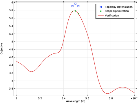
In the Settings window for Global, click Add Expression in the upper-right corner of the y-Axis Data section. From the menu, choose Component 1 (comp1) > Definitions > obj - Objective - V/m.
3
Locate the y-Axis Data section. In the table, enter the following settings:
4
Click to expand the Coloring and Style section. Find the Line style subsection. From the Line list, choose None.
5
Find the Line markers subsection. From the Marker list, choose Square.
Global 2
1
Right-click Global 1 and choose Duplicate.
2
In the Settings window for Global, locate the Data section.
3
From the Dataset list, choose Study 2: Shape Optimization/Solution 6 (5) (sol6).
4
Locate the y-Axis Data section. In the table, enter the following settings:
5
Locate the x-Axis Data section. From the Parameter list, choose Expression.
6
In the Expression text field, type lambda0.
7
Locate the Coloring and Style section. Find the Line markers subsection. From the Marker list, choose Point.
Global 3
1
Right-click Global 2 and choose Duplicate.
2
In the Settings window for Global, locate the Data section.
3
From the Dataset list, choose Study 3: Verification/Solution 7 (7) (sol7).
4
Locate the y-Axis Data section. In the table, enter the following settings:
5
Locate the Coloring and Style section. Find the Line style subsection. From the Line list, choose Solid.
6
Find the Line markers subsection. From the Marker list, choose None.
7
Click the  Zoom Extents button in the Graphics toolbar.
8
In the Verification toolbar, click  Plot.
Revolution 2D 2
1
In the Model Builder window, under Results > Datasets click Revolution 2D 2.
2
In the Settings window for Revolution 2D, click to collapse the Axis Data section.
3
Locate the Data section. From the Dataset list, choose Filter 1.
4
Click to expand the Revolution Layers section. In the Start angle text field, type 250.
5
In the Revolution angle text field, type 270.
Revolution 2D 1
1
In the Model Builder window, click Revolution 2D 1.
2
In the Settings window for Revolution 2D, locate the Revolution Layers section.
3
In the Start angle text field, type 250.
4
In the Revolution angle text field, type 270.
Selection
1
Right-click Revolution 2D 1 and choose Selection.
2
In the Settings window for Selection, locate the Geometric Entity Selection section.
3
From the Geometric entity level list, choose Domain.
4
Thumbnail
1
In the Results toolbar, click  3D Plot Group.
2
In the Settings window for 3D Plot Group, type Thumbnail in the Label text field.
Volume 1
1
Right-click Thumbnail and choose Volume.
2
In the Settings window for Volume, locate the Coloring and Style section.
3
Clear the Color legend checkbox.
Filter 1
1
Right-click Volume 1 and choose Filter.
2
In the Settings window for Filter, locate the Element Selection section.
3
In the Logical expression for inclusion text field, type 0.5<centroid(genext2(theta_m)).
Transparency 1
1
In the Model Builder window, right-click Volume 1 and choose Transparency.
2
In the Settings window for Transparency, locate the Transparency section.
3
Find the Transparency subsection. In the Transparency text field, type 1.
Isosurface 1
1
In the Model Builder window, right-click Thumbnail and choose Isosurface.
2
In the Settings window for Isosurface, locate the Expression section.
3
In the Expression text field, type if(0.5*lens_H<Z || 0<rev1phi,ewfd.normE,nan).
4
Locate the Levels section. In the Total levels text field, type 8.
Color Expression 1
1
Right-click Isosurface 1 and choose Color Expression.
2
In the Settings window for Color Expression, locate the Coloring and Style section.
3
From the Color table list, choose Thermal.
4
From the Color table transformation list, choose Reverse.
Visual Effects 1
1
In the Model Builder window, right-click Isosurface 1 and choose Visual Effects.
2
In the Settings window for Visual Effects, locate the Visual Effects section.
3
Find the Direct shadows subsection. From the Mode list, choose Manual.
4
Clear the Casts shadows checkbox.
Transformation 1
1
Right-click Isosurface 1 and choose Transformation.
2
In the Settings window for Transformation, locate the Transformation section.
3
Select the Rotate checkbox.
4
In the Angle text field, type 1.
Surface 1
1
In the Model Builder window, right-click Thumbnail and choose Surface.
2
In the Settings window for Surface, locate the Expression section.
3
In the Expression text field, type 1.
4
Locate the Coloring and Style section. From the Coloring list, choose Uniform.
5
From the Color list, choose Blue.
6
Click to expand the Quality section. From the Evaluation settings list, choose Manual.
7
From the Smoothing list, choose None.
Filter 1
1
Right-click Surface 1 and choose Filter.
2
In the Settings window for Filter, locate the Element Selection section.
3
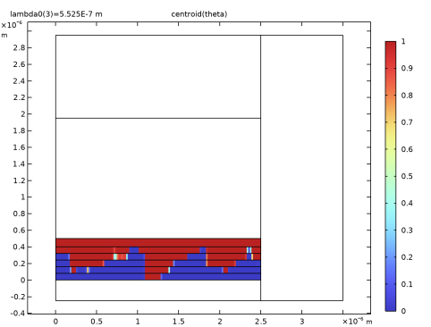
In the Logical expression for inclusion text field, type (0.5<centroid(theta)) && rev1phi<-220/360*pi.
4
In the Thumbnail toolbar, click  Plot.
5
Click the  Zoom Extents button in the Graphics toolbar.
Disable the interfaces of the second component in the first study.
Study 1: Topology Optimization
Topology Optimization
1
In the Model Builder window, under Study 1: Topology Optimization click Topology Optimization.
2
In the Settings window for Topology Optimization, locate the Control Variables section.
3
In the table, clear the Solve for checkbox for Transformation 1.
Step 1: Wavelength Domain
1
In the Model Builder window, click Step 1: Wavelength Domain.
2
In the Settings window for Wavelength Domain, locate the Physics and Variables Selection section.
3
In the Solve for column of the table, clear the checkbox for Component 2: Verification (comp2).
Geometry Modeling Instructions
From the File menu, choose New.
New
In the New window, click  Blank Model.
Global Definitions
Parameters 1
1
In the Model Builder window, under Global Definitions click Parameters 1.
2
In the Settings window for Parameters, locate the Parameters section.
3
Add Component
In the Home toolbar, click  Add Component and choose 2D Axisymmetric.
Geometry 1
Rectangle 1 (r1)
1
In the Geometry toolbar, click  Rectangle.
2
In the Settings window for Rectangle, locate the Size and Shape section.
3
In the Width text field, type 0.5*lens_l.
4
In the Height text field, type lens_H.
5
Click to expand the Layers section. In the table, enter the following settings:
6
Locate the Selections of Resulting Entities section. Select the Resulting objects selection checkbox.
Point 1 (pt1)
1
In the Geometry toolbar, click  Point.
2
In the Settings window for Point, locate the Point section.
3
In the z text field, type lens_F+lens_H/2+d_src_lens.
4
Locate the Selections of Resulting Entities section. Select the Resulting objects selection checkbox.
Rectangle 2 (r2)
1
In the Geometry toolbar, click  Rectangle.
2
In the Settings window for Rectangle, locate the Size and Shape section.
3
In the Width text field, type d_PML.
4
In the Height text field, type cell_H-d_PML.
5
Locate the Position section. In the r text field, type lens_l/2.
6
In the z text field, type -d_src_lens.
Rectangle 3 (r3)
1
In the Model Builder window, under Component 1 (comp1) > Geometry 1 right-click Rectangle 1 (r1) and choose Duplicate.
2
In the Settings window for Rectangle, locate the Size and Shape section.
3
In the Height text field, type cell_H-d_PML.
4
Locate the Position section. In the z text field, type -d_src_lens.
5
Locate the Layers section. In the table, enter the following settings:
Rectangle 4 (r4)
1
In the Geometry toolbar, click  Rectangle.
2
In the Settings window for Rectangle, locate the Size and Shape section.
3
In the Width text field, type 0.5*lens_l.
4
In the Height text field, type (lens_H-lens_minH)/layers.
5
Locate the Selections of Resulting Entities section. Select the Resulting objects selection checkbox.
Control layers
1
In the Geometry toolbar, click  Selections and choose Box Selection.
2
In the Settings window for Box Selection, type Control layers in the Label text field.
3
Locate the Geometric Entity Level section. From the Level list, choose Boundary.
4
Locate the Box Limits section. In the z minimum text field, type -eps.
5
In the z maximum text field, type eps.
6
Locate the Output Entities section. From the Include entity if list, choose Entity inside box.
Array 1 (arr1)
1
In the Geometry toolbar, click  Transforms and choose Array.
2
In the Settings window for Array, locate the Input section.
3
From the Input objects list, choose Rectangle 4.
4
Locate the Size section. In the z size text field, type layers.
5
Locate the Displacement section. In the z text field, type (lens_H-lens_minH)/layers.
Form Union (fin)
1
In the Model Builder window, click Form Union (fin).
2
In the Settings window for Form Union/Assembly, click  Build Selected.
Symmetry/Roller
1
In the Geometry toolbar, click  Selections and choose Box Selection.
2
In the Settings window for Box Selection, type Symmetry/Roller in the Label text field.
3
Locate the Geometric Entity Level section. From the Level list, choose Boundary.
4
Locate the Box Limits section. In the r minimum text field, type 0.1*lens_l.
5
In the r maximum text field, type 0.4*lens_l.
6
In the z minimum text field, type -0.001*lens_H.
7
In the z maximum text field, type 1.001*lens_H.
Source
1
In the Geometry toolbar, click  Selections and choose Box Selection.
2
In the Settings window for Box Selection, type Source in the Label text field.
3
Locate the Geometric Entity Level section. From the Level list, choose Boundary.
4
Locate the Box Limits section. In the z maximum text field, type -eps.
5
Locate the Output Entities section. From the Include entity if list, choose Entity inside box.
PML
1
In the Geometry toolbar, click  Selections and choose Box Selection.
2
In the Settings window for Box Selection, type PML in the Label text field.
3
Locate the Box Limits section. In the r minimum text field, type lens_l*0.49.
4
In the z minimum text field, type cell_H-lens_H/2-3*d_PML/2.
Fixed Lens
1
In the Model Builder window, under Component 1 (comp1) > Geometry 1 right-click Source (boxsel3) and choose Duplicate.
2
In the Settings window for Box Selection, type Fixed Lens in the Label text field.
3
Locate the Geometric Entity Level section. From the Level list, choose Domain.
4
Locate the Box Limits section. In the z minimum text field, type lens_H-1.01*lens_minH.
5
In the z maximum text field, type 1.01*lens_H.
6
Click the  Zoom Extents button in the Graphics toolbar.
The model geometry is now complete.