PDF

Optimization of an Extruded MBB Beam
Introduction
Topology and shape optimization can be used to find and improve the design of products, but sometimes manufacturing constraints dictate that the design most be invariant in one of the dimensions, that is, an extruded geometry is desired. If 3-dimensional effects play little role, a 2D optimization can be used. Otherwise, one has to perform a 3D simulation and restrict the optimization to preserve the extruded property of the geometry.
This model is inspired by Topology Optimization of an MBB Beam, but the geometry is forced to be invariant in the z direction. The result is transferred to a second component in which shape optimization is performed, while still preserving the invariance in the z direction.
Model Definition
The model uses the Density Model feature to setup the topology optimization with an extrusion manufacturing constraint.
The shape optimization combines a Free Shape Shell feature with a General Extrusion operator, so that the deformation is only occurs in the xy-plane and does not vary in the z-coordinate.
Results and Discussion
The result of the topology optimization is shown in Figure 1. The model accounts for out-of-plane displacements, but the design is identical to the 2D result in the model Topology Optimization of an MBB Beam.
Figure 1: The filtered material volume factor is plotted on the z symmetry plane associated with the Density Model. An extrusion operator is used to transfer the variable to the volume.
The General Extrusion operator used for the shape optimization will be more robust if it is used on an extruded design. There are several ways to achieve this, but in this model we will combine a Filter dataset, a Mesh part and a geometry Import feature to transfer a 2D version of the design. This is then extruded as shown in Figure 2.
Figure 2: ‘The topology optimized design has been transferred to a second component using an extrusion operator and a filter dataset pointing to a cut plane dataset. Note the shell representation in the background which is used to setup the shape optimization.
Finally, the result of the shape optimization is shown in Figure 3 as the initial volume in gray on top of the optimized volume in red (transparency is enabled). The 90-degree angle near the top boundary is removed, because it is an artifact of the Helmholtz filter and thus not optimal (similar to Shape Optimization of an MBB Beam).
Figure 3: The plot shows the initial and optimized geometries in gray and red, respectively.
Notes About the COMSOL Implementation
This model combines the Topology Optimization, Shape Optimization, Solid Mechanics and Deforming Geometry interfaces. The model uses a Filter dataset to transfer the geometry between components. An alternatively method is to export the edges as a text file with a section-wise format and import them as an interpolation curve. The interpolation curve has a parameter that can be used to straighten out the wiggles, but this approach requires more geometry operations to identify and delete the void domain.
Finally, the plot with transparency suffers from z-fighting artifacts on the Symmetry/Roller boundaries, but this is rectified by shrinking one of the volumes slightly.
Application Library path: Optimization_Module/Design_Optimization/mbb_beam_extruded_optimization
Modeling Instructions
From the File menu, choose New.
New
In the New window, click  Model Wizard.
Model Wizard
1
In the Model Wizard window, click  3D.
2
In the Select Physics tree, select Structural Mechanics > Solid Mechanics (solid).
3
Click Add.
4
Click  Study.
5
In the Select Study tree, select Preset Studies for Selected Physics Interfaces > Optimization > Topology Optimization, Stationary.
6
Global Definitions
Parameters 1
1
In the Model Builder window, under Global Definitions click Parameters 1.
2
In the Settings window for Parameters, locate the Parameters section.
3
Geometry 1
Work Plane 1 (wp1)
In the Geometry toolbar, click  Work Plane.
Work Plane 1 (wp1) > Plane Geometry
In the Model Builder window, click Plane Geometry.
Work Plane 1 (wp1) > Rectangle 1 (r1)
1
In the Work Plane toolbar, click  Rectangle.
2
In the Settings window for Rectangle, locate the Size and Shape section.
3
In the Width text field, type a.
4
In the Height text field, type b.
Work Plane 1 (wp1) > Point 1 (pt1)
1
In the Work Plane toolbar, click  Point.
2
In the Settings window for Point, locate the Point section.
3
In the yw text field, type L1.
Work Plane 1 (wp1) > Point 2 (pt2)
1
In the Work Plane toolbar, click  Point.
2
In the Settings window for Point, locate the Point section.
3
In the xw text field, type a-L1/2.
4
In the yw text field, type b.
Extrude 1 (ext1)
1
In the Model Builder window, under Component 1 (comp1) > Geometry 1 right-click Work Plane 1 (wp1) and choose Extrude.
2
In the Settings window for Extrude, locate the Distances section.
3
Symmetry z Boundary
1
In the Geometry toolbar, click  Selections and choose Box Selection.
2
In the Settings window for Box Selection, type Symmetry z Boundary in the Label text field.
3
Locate the Geometric Entity Level section. From the Level list, choose Boundary.
4
Locate the Box Limits section. In the z maximum text field, type c*0.001.
5
Locate the Output Entities section. From the Include entity if list, choose Entity inside box.
6
In the Geometry toolbar, click  Build All.
The model geometry is now complete.
Materials
Topology Link 1 (toplnk1)
In the Model Builder window, under Component 1 (comp1) > Materials right-click Topology Link 1 (toplnk1) and choose Delete.
Add Material
1
In the Materials toolbar, click  Add Material to open the Add Material window.
2
Go to the Add Material window.
3
In the tree, select Built-in > Structural steel.
4
Click the Add to Global Materials button in the window toolbar.
5
In the Materials toolbar, click  Add Material to close the Add Material window.
Solid Mechanics (solid)
Roller 1
1
In the Physics toolbar, click  Boundaries and choose Roller.
2
Prescribed Displacement 1
1
In the Physics toolbar, click  Boundaries and choose Prescribed Displacement.
2
3
In the Settings window for Prescribed Displacement, locate the Prescribed Displacement section.
4
From the Displacement in y direction list, choose Prescribed.
This is effectively a roller condition along the x-axis, but it is applied on a vertical boundary to avoid bending stiffness.
Boundary Load 1
1
In the Physics toolbar, click  Boundaries and choose Boundary Load.
2
3
In the Settings window for Boundary Load, locate the Force section.
4
From the Load type list, choose Total force.
5
Specify the Ftot vector as
Mesh 1
Create a swept mesh along the extrusion direction of the geometry.
Free Triangular 1
1
In the Mesh toolbar, click  More Generators and choose Free Triangular.
2
In the Settings window for Free Triangular, locate the Boundary Selection section.
3
From the Selection list, choose Symmetry z Boundary.
Size
1
In the Model Builder window, click Size.
2
In the Settings window for Size, locate the Element Size section.
3
From the Predefined list, choose Extremely fine.
Swept 1
1
In the Mesh toolbar, click  Swept.
2
In the Settings window for Swept, click  Build All.
Topology Optimization
Density Model 1 (dtopo1)
1
In the Model Builder window, under Component 1 (comp1) > Topology Optimization click Density Model 1 (dtopo1).
2
In the Settings window for Density Model, click to expand the Manufacturing Constraints section.
3
From the Manufacturing constraints list, choose Extrusion.
4
Click to expand the Extruded Boundary section. From the Selection list, choose Symmetry z Boundary.
5
Locate the Control Variable Initial Value section. In the θ0 text field, type volfrac.
Materials
Topology Link 1 (toplnk1)
1
In the Model Builder window, under Component 1 (comp1) right-click Materials and choose More Materials > Topology Link.
2
In the Settings window for Topology Link, locate the Geometric Entity Selection section.
3
From the Selection list, choose All domains.
4
Locate the Link Settings section. From the Topology source list, choose Density Model 1 (dtopo1).
Study 1: Topology Optimization
1
In the Model Builder window, click Study 1.
2
In the Settings window for Study, type Study 1: Topology Optimization in the Label text field.
Initialize the study to create a default plot to display while solving.
3
In the Study toolbar, click  Get Initial Value.
The surface plot can visualize intermediate design variables, but now that the optimization has finished, it makes sense to change the filter dataset so that the threshold volume plot represents the optimized geometry.
Topology Optimization
1
In the Model Builder window, under Study 1: Topology Optimization click Topology Optimization.
2
In the Settings window for Topology Optimization, locate the Optimization Solver section.
3
In the Maximum number of iterations text field, type 25.
4
Locate the Constraints section. In the table, enter the following settings:
5
Click to expand the Output section. Select the Plot checkbox.
6
7
In the Study toolbar, click  Compute.
Results
In the Model Builder window, expand the Results > Topology Optimization node.
Surface 1
1
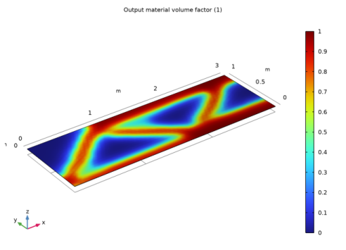
In the Model Builder window, expand the Results > Topology Optimization > Output material volume factor node, then click Surface 1.
2
In the Output material volume factor toolbar, click  Plot.
Threshold
1
In the Model Builder window, under Results > Topology Optimization click Threshold.
2
In the Threshold toolbar, click  Plot.
Create a Cut Plane dataset for a 2D plot group, so that the design can be exported.
Cut Plane 1
1
In the Model Builder window, expand the Results > Datasets node.
2
Right-click Results > Datasets and choose Cut Plane.
3
In the Settings window for Cut Plane, locate the Data section.
4
From the Dataset list, choose Study 1: Topology Optimization/Solution 1 (sol1).
5
Locate the Plane Data section. From the Plane list, choose XY-planes.
Filter 2
1
In the Results toolbar, click  More Datasets and choose Filter.
2
In the Settings window for Filter, locate the Data section.
3
From the Dataset list, choose Cut Plane 1.
4
Locate the Expression section. In the Expression text field, type dtopo1.theta_f.
5
Locate the Filter section. In the Lower bound text field, type 0.5.
6
Locate the Evaluation section. From the Smoothing list, choose None.
7
Clear the Use derivatives checkbox.
8
Right-click Filter 2 and choose Create Mesh Part.
Mesh Part 1
1
In the Model Builder window, under Global Definitions > Mesh Parts right-click Mesh Part 1 and choose Build All.
2
Right-click Global Definitions > Mesh Parts > Mesh Part 1 and choose Create Geometry.
Geometry 2
Import 1 (imp1)
1
In the Settings window for Import, locate the Simplify and Repair section.
2
Clear the Form solids from surface objects checkbox.
3
Click to expand the Selections of Resulting Entities section. Select the Resulting objects selection checkbox.
4
From the Show in physics list, choose Boundary selection.
Extrude 1 (ext1)
1
In the Geometry toolbar, click  Extrude.
2
In the Settings window for Extrude, locate the General section.
3
From the Input faces list, choose Import 1.
4
From the Input object handling list, choose Keep.
5
Locate the Distances section. In the table, enter the following settings:
6
Select the Reverse direction checkbox.
7
Click  Build Selected.
Move 1 (mov1)
1
In the Geometry toolbar, click  Transforms and choose Move.
2
In the Settings window for Move, locate the Input section.
3
From the Input objects list, choose Import 1.
4
Locate the Displacement section. In the z text field, type -c.
5
Locate the Selections of Resulting Entities section. Select the Resulting objects selection checkbox.
6
From the Show in physics list, choose Boundary selection.
Line Segment 1 (ls1)
1
In the Geometry toolbar, click  More Primitives and choose Line Segment.
2
In the Settings window for Line Segment, locate the Starting Point section.
3
From the Specify list, choose Coordinates.
4
In the y text field, type L1.
5
Locate the Endpoint section. From the Specify list, choose Coordinates.
6
In the y text field, type L1.
7
In the z text field, type c.
Line Segment 2 (ls2)
1
In the Geometry toolbar, click  More Primitives and choose Line Segment.
2
In the Settings window for Line Segment, locate the Starting Point section.
3
From the Specify list, choose Coordinates.
4
In the x text field, type a-L1/2.
5
In the y text field, type b.
6
Locate the Endpoint section. From the Specify list, choose Coordinates.
7
In the x text field, type a-L1/2.
8
In the y text field, type b.
9
In the z text field, type c.
10
In the Geometry toolbar, click  Build All.
The geometry should now look like that in Figure 1.
Line Segment 3 (ls3)
1
In the Geometry toolbar, click  More Primitives and choose Line Segment.
2
In the Settings window for Line Segment, locate the Starting Point section.
3
From the Specify list, choose Coordinates.
4
Locate the Endpoint section. From the Specify list, choose Coordinates.
5
Locate the Starting Point section. In the x text field, type a-L1/2.
6
In the y text field, type b.
7
In the z text field, type -c.
8
Locate the Endpoint section. In the x text field, type a.
9
In the y text field, type b.
10
In the z text field, type -c.
11
Locate the Selections of Resulting Entities section. Select the Resulting objects selection checkbox.
Line Segment 4 (ls4)
1
In the Geometry toolbar, click  More Primitives and choose Line Segment.
2
In the Settings window for Line Segment, locate the Starting Point section.
3
From the Specify list, choose Coordinates.
4
Locate the Endpoint section. From the Specify list, choose Coordinates.
5
Locate the Starting Point section. In the x text field, type 0.
6
In the y text field, type 0.
7
In the z text field, type -c.
8
Locate the Endpoint section. In the x text field, type 0.
9
In the y text field, type L1.
10
In the z text field, type -c.
11
Locate the Selections of Resulting Entities section. Select the Resulting objects selection checkbox.
Form Union (fin)
1
In the Model Builder window, click Form Union (fin).
2
In the Settings window for Form Union/Assembly, click  Build Selected.
Symmetry x
1
In the Geometry toolbar, click  Selections and choose Box Selection.
2
In the Settings window for Box Selection, type Symmetry x in the Label text field.
3
Locate the Geometric Entity Level section. From the Level list, choose Boundary.
4
Locate the Box Limits section. In the x minimum text field, type 0.999*a.
5
Locate the Output Entities section. From the Include entity if list, choose Entity inside box.
Symmetry x edge 1
1
Right-click Symmetry x and choose Duplicate.
2
In the Settings window for Box Selection, type Symmetry x edge 1 in the Label text field.
3
Locate the Geometric Entity Level section. From the Level list, choose Edge.
4
Click  Build Selected.
Roller support
1
In the Geometry toolbar, click  Selections and choose Box Selection.
2
In the Settings window for Box Selection, type Roller support in the Label text field.
3
Locate the Geometric Entity Level section. From the Level list, choose Boundary.
4
Locate the Box Limits section. In the x maximum text field, type 0.001*a.
5
In the y maximum text field, type 1.01*L1.
6
Locate the Output Entities section. From the Include entity if list, choose Entity inside box.
Symmetry x edge 2
1
Right-click Roller support and choose Duplicate.
2
In the Settings window for Box Selection, locate the Geometric Entity Level section.
3
From the Level list, choose Edge.
4
In the Label text field, type Symmetry x edge 2.
5
Locate the Box Limits section. In the y minimum text field, type 0.99*L1.
6
In the y maximum text field, type Inf.
7
Click  Build Selected.
Load boundary
1
In the Geometry toolbar, click  Selections and choose Box Selection.
2
In the Settings window for Box Selection, type Load boundary in the Label text field.
3
Locate the Geometric Entity Level section. From the Level list, choose Boundary.
4
Locate the Box Limits section. In the x minimum text field, type a-0.51*L1.
5
In the y minimum text field, type 0.99*b.
6
Locate the Output Entities section. From the Include entity if list, choose Entity inside box.
Symmetry y edge 1
1
Right-click Load boundary and choose Duplicate.
2
In the Settings window for Box Selection, type Symmetry y edge 1 in the Label text field.
3
Locate the Geometric Entity Level section. From the Level list, choose Edge.
4
Locate the Box Limits section. In the x minimum text field, type -Inf.
Symmetry y edge 2
1
Right-click Symmetry y edge 1 and choose Duplicate.
2
In the Settings window for Box Selection, type Symmetry y edge 2 in the Label text field.
3
Locate the Box Limits section. In the y minimum text field, type -Inf.
4
In the y maximum text field, type 0.01*b.
5
Click  Build Selected.
Fixed edges
1
In the Geometry toolbar, click  Selections and choose Union Selection.
2
In the Settings window for Union Selection, locate the Geometric Entity Level section.
3
From the Level list, choose Edge.
4
In the Label text field, type Fixed edges.
5
Locate the Input Entities section. Click  Add.
6
In the Add dialog, in the Selections to add list, choose Line Segment 3 and Line Segment 4.
7
Symmetry y edge
1
In the Geometry toolbar, click  Selections and choose Union Selection.
2
In the Settings window for Union Selection, type Symmetry y edge in the Label text field.
3
In the Model Builder window, click Symmetry y edge (unisel2).
4
In the Label text field, type Symmetry y edge.
5
Locate the Geometric Entity Level section. From the Level list, choose Edge.
6
Locate the Input Entities section. Click  Add.
7
In the Add dialog, in the Selections to add list, choose Symmetry y edge 1 and Symmetry y edge 2.
8
Symmetry x edge
1
In the Geometry toolbar, click  Selections and choose Union Selection.
2
In the Settings window for Union Selection, type Symmetry x edge in the Label text field.
3
Locate the Geometric Entity Level section. From the Level list, choose Edge.
4
Locate the Input Entities section. Click  Add.
5
In the Add dialog, in the Selections to add list, choose Symmetry x edge 1 and Symmetry x edge 2.
6
Component 1: Topology Optimization
1
In the Model Builder window, click Component 1 (comp1).
2
In the Settings window for Component, type Component 1: Topology Optimization in the Label text field.
Component 2: Shape Optimization
1
In the Model Builder window, click Component 2 (comp2).
2
In the Settings window for Component, type Component 2: Shape Optimization in the Label text field.
Global Definitions
Parameters 1
Add the shape optimization parameters.
1
In the Model Builder window, under Global Definitions click Parameters 1.
2
In the Settings window for Parameters, locate the Parameters section.
3
Component 2: Shape Optimization (comp2)
Free Shape Shell 1
1
In the Physics toolbar, click  Optimization and choose Shape Optimization, Shell.
2
In the Settings window for Free Shape Shell, locate the Boundary Selection section.
3
From the Selection list, choose Move 1.
4
Locate the Control Variable Settings section. From the dmax list, choose User defined.
5
6
Locate the Filtering section. From the Rmin list, choose User defined.
7
Symmetry/Roller 1
1
In the Shape Optimization toolbar, click  Symmetry/Roller.
2
In the Settings window for Symmetry/Roller, locate the Geometric Entity Selection section.
3
From the Geometric entity level list, choose Edge.
4
From the Selection list, choose Symmetry y edge.
5
Locate the Prescribed Normal Vector section. Specify the n vector as
Symmetry/Roller 2
1
Right-click Symmetry/Roller 1 and choose Duplicate.
2
In the Settings window for Symmetry/Roller, locate the Geometric Entity Selection section.
3
From the Selection list, choose Symmetry x edge.
4
Locate the Prescribed Normal Vector section. Specify the n vector as
Fixed Edge 1
1
In the Shape Optimization toolbar, click  Fixed Edge.
2
In the Settings window for Fixed Edge, locate the Edge Selection section.
3
From the Selection list, choose Fixed edges.
Add Physics
1
In the Shape Optimization toolbar, click  Add Physics to open the Add Physics window.
2
Go to the Add Physics window.
3
In the tree, select Structural Mechanics > Solid Mechanics (solid).
4
Find the Physics interfaces in study subsection. In the table, clear the Solve checkbox for Study 1: Topology Optimization.
5
Click the Add to Component 2: Shape Optimization button in the window toolbar.
6
In the Home toolbar, click  Add Physics to close the Add Physics window.
Materials
Material Link 1 (matlnk1)
In the Model Builder window, under Component 2: Shape Optimization (comp2) right-click Materials and choose More Materials > Material Link.
Study 1: Topology Optimization
Topology Optimization
1
In the Settings window for Topology Optimization, locate the Control Variables section.
2
In the table, clear the Solve for checkbox for Free Shape Shell 1.
Definitions (comp2)
Add a nonlocal integration coupling to enforce the volume constraint.
Integration 1 (intop1)
1
In the Definitions toolbar, click  Nonlocal Couplings and choose Integration.
2
In the Settings window for Integration, locate the Source Selection section.
3
From the Selection list, choose All domains.
Once again use an extrusion operator to transfer the filtered field from the boundary to the domain.
General Extrusion 1 (genext1)
1
In the Definitions toolbar, click  Nonlocal Couplings and choose General Extrusion.
2
In the Settings window for General Extrusion, locate the Source Selection section.
3
From the Geometric entity level list, choose Boundary.
4
From the Selection list, choose Move 1.
5
Locate the Destination Map section. In the x-expression text field, type Xg.
6
In the y-expression text field, type Yg.
7
In the z-expression text field, type -c.
8
Locate the Source section. From the Source frame list, choose Geometry  (Xg, Yg, Zg).
Deformed Geometry
Prescribed Deformation 1
1
In the Deformed Geometry toolbar, click  Prescribed Deformation.
2
In the Settings window for Prescribed Deformation, locate the Geometric Entity Selection section.
3
From the Selection list, choose All domains.
4
Locate the Prescribed Deformation section. Specify the dx vector as
Solid Mechanics 2 (solid2)
Roller 1
1
In the Physics toolbar, click  Boundaries and choose Roller.
2
In the Settings window for Roller, locate the Boundary Selection section.
3
From the Selection list, choose Symmetry x.
Roller 2
1
In the Physics toolbar, click  Boundaries and choose Roller.
2
In the Settings window for Roller, locate the Boundary Selection section.
3
From the Selection list, choose Import 1.
Prescribed Displacement 1
1
In the Physics toolbar, click  Boundaries and choose Prescribed Displacement.
2
In the Settings window for Prescribed Displacement, locate the Boundary Selection section.
3
From the Selection list, choose Roller support.
4
Locate the Prescribed Displacement section. From the Displacement in y direction list, choose Prescribed.
Boundary Load 1
1
In the Physics toolbar, click  Boundaries and choose Boundary Load.
2
In the Settings window for Boundary Load, locate the Boundary Selection section.
3
From the Selection list, choose Load boundary.
4
Locate the Force section. From the Load type list, choose Total force.
5
Specify the Ftot vector as
Mesh 2
Once again create a swept mesh along the extrusion direction of the geometry.
Free Triangular 1
1
In the Mesh toolbar, click  More Generators and choose Free Triangular.
2
In the Settings window for Free Triangular, locate the Boundary Selection section.
3
From the Selection list, choose Import 1.
Size
1
In the Model Builder window, click Size.
2
In the Settings window for Size, locate the Element Size section.
3
From the Predefined list, choose Extremely fine.
4
Click to expand the Element Size Parameters section. In the Curvature factor text field, type 2.
Swept 1
1
In the Mesh toolbar, click  Swept.
2
In the Settings window for Swept, click  Build All.
Add Study
1
In the Home toolbar, click  Add Study to open the Add Study window.
2
Go to the Add Study window.
3
Find the Physics interfaces in study subsection. In the table, clear the Solve checkbox for Solid Mechanics (solid).
4
Find the Studies subsection. In the Select Study tree, select General Studies > Stationary.
5
Click the Add Study button in the window toolbar.
6
In the Home toolbar, click  Add Study to close the Add Study window.
Study 1: Topology Optimization
Step 1: Stationary
1
In the Settings window for Stationary, locate the Physics and Variables Selection section.
2
In the Solve for column of the table, under Component 2: Shape Optimization (comp2), clear the checkbox for Deformed Geometry.
Study 2: Shape Optimization
1
In the Model Builder window, click Study 2.
2
In the Settings window for Study, type Study 2: Shape Optimization in the Label text field.
Shape Optimization
1
In the Study toolbar, click  Optimization and choose Shape Optimization.
2
In the Settings window for Shape Optimization, locate the Optimization Solver section.
3
In the Maximum number of iterations text field, type 20.
4
Clear the Move limits checkbox.
5
Click Replace Expression in the upper-right corner of the Objective Function section. From the menu, choose Component 2: Shape Optimization (comp2) > Solid Mechanics 2 > Global > comp2.solid2.Ws_tot - Total elastic strain energy - J.
6
Locate the Objective Function section. Find the Objective settings subsection. From the Objective scaling list, choose Initial solution based.
7
Locate the Control Variables section. In the table, clear the Solve for checkbox for Density Model 1 (dtopo1).
8
Click Add Expression in the upper-right corner of the Constraints section. From the menu, choose Component 2: Shape Optimization (comp2) > Definitions > Nonlocal couplings > comp2.intop1(expr) - Integration 1.
9
Locate the Constraints section. In the table, enter the following settings:
Step 1: Stationary
1
In the Model Builder window, click Step 1: Stationary.
2
In the Settings window for Stationary, locate the Physics and Variables Selection section.
3
In the Solve for column of the table, under Component 1: Topology Optimization (comp1), clear the checkbox for Topology Optimization.
Initialize the study to create a plot for use while solving.
4
In the Study toolbar, click  Get Initial Value.
Shape Optimization
1
In the Model Builder window, click Shape Optimization.
2
In the Settings window for Shape Optimization, click to expand the Output section.
3
Select the Plot checkbox.
4
5
In the Study toolbar, click  Compute.
Results
Deformed Geometry, Topology Optimization 1
Right-click and choose Delete.
Create a dataset in the geometry frame, so that the initial and optimized volumes can be plotted on top of each other. The plot illustrates the shape change in an alternative way, but it only makes sense with transparency enabled.
Study 1: Topology Optimization/Solution 1 (4) (sol1)
1
In the Results toolbar, click  More Datasets and choose Solution.
2
In the Settings window for Solution, locate the Solution section.
3
From the Solution list, choose Solution 2 (sol2).
4
From the Component list, choose Component 2: Shape Optimization (comp2).
5
From the Frame list, choose Geometry  (Xg, Yg, Zg).
Volumetric (for transparent view)
1
In the Results toolbar, click  3D Plot Group.
2
In the Settings window for 3D Plot Group, locate the Data section.
3
From the Dataset list, choose Study 2: Shape Optimization/Solution 2 (3) (sol2).
4
Locate the Plot Settings section. Clear the Plot dataset edges checkbox.
5
In the Label text field, type Volumetric (for transparent view).
Volume 1
1
Right-click Volumetric (for transparent view) and choose Volume.
2
In the Settings window for Volume, locate the Coloring and Style section.
3
From the Coloring list, choose Uniform.
Volume 2
1
In the Model Builder window, right-click Volumetric (for transparent view) and choose Volume.
2
In the Settings window for Volume, locate the Data section.
3
From the Dataset list, choose Study 2: Shape Optimization/Solution 2 (4) (sol2).
4
Locate the Coloring and Style section. From the Coloring list, choose Uniform.
5
From the Color list, choose Gray.
6
Click the  Transparency button in the Graphics toolbar.
7
In the Volumetric (for transparent view) toolbar, click  Plot.
There are some z-fighting artifacts on the Symmetry/Roller boundaries, but this can be avoided by shrinking one of the plots slightly.
Deformation 1
1
In the Model Builder window, right-click Volume 1 and choose Deformation.
2
In the Settings window for Deformation, locate the Expression section.
3
In the X-component text field, type -1e-3*(Xg/a-0.5).
4
In the Y-component text field, type -1e-3*(Yg/b-0.5).
5
In the Z-component text field, type -1e-3*(Zg/c-0.5).
6
Locate the Scale section.
7
Select the Scale factor checkbox. In the associated text field, type 1.
8
In the Volumetric (for transparent view) toolbar, click  Plot.
Stress (solid) Topology Optimization
1
In the Model Builder window, under Results click Stress (solid).
2
In the Settings window for 3D Plot Group, type Stress (solid) Topology Optimization in the Label text field.