|
|
|
|
1
|
|
2
|
|
3
|
Click Add.
|
|
4
|
Click
|
|
5
|
In the Select Study tree, select Preset Studies for Selected Physics Interfaces > Optimization > Topology Optimization, Stationary.
|
|
6
|
Click
|
|
1
|
|
2
|
Browse to the model’s Application Libraries folder and double-click the file hook_optimization_stl_geom_sequence.mph.
|
|
3
|
|
4
|
|
5
|
|
1
|
|
2
|
|
1
|
|
2
|
|
1
|
|
2
|
|
3
|
|
1
|
|
2
|
|
3
|
Click the Custom button.
|
|
4
|
|
5
|
|
6
|
Click
|
|
1
|
|
2
|
Go to the Add Material window.
|
|
3
|
|
4
|
Click the Add to Global Materials button in the window toolbar.
|
|
5
|
|
1
|
|
2
|
|
3
|
|
1
|
In the Model Builder window, under Component 1 (comp1) > Topology Optimization click Density Model 1 (dtopo1).
|
|
2
|
|
3
|
|
4
|
|
5
|
In the text field, type Lmin.
|
|
6
|
Click to expand the Manufacturing Constraints section. From the Manufacturing constraints list, choose Milling.
|
|
8
|
|
10
|
|
11
|
|
12
|
|
1
|
|
2
|
|
3
|
|
1
|
|
2
|
In the Settings window for Prescribed Material Boundary, locate the Geometric Entity Selection section.
|
|
3
|
|
1
|
|
2
|
|
3
|
|
1
|
|
2
|
|
3
|
|
1
|
|
2
|
|
3
|
|
4
|
|
5
|
|
1
|
|
2
|
|
3
|
|
4
|
|
5
|
|
6
|
|
1
|
|
2
|
|
3
|
|
4
|
|
1
|
|
2
|
|
1
|
|
2
|
|
3
|
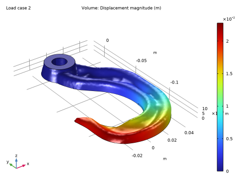
Select the Define load cases checkbox.
|
|
4
|
Click
|
|
5
|
Click
|
|
7
|
|
1
|
|
2
|
|
3
|
|
4
|
|
1
|
|
2
|
|
3
|
|
1
|
|
2
|
|
3
|
|
4
|
Locate the Constraints section. In the table, enter the following settings:
|
|
5
|
|
6
|
|
7
|
|
1
|
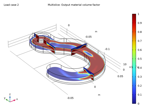
In the Model Builder window, under Results > Topology Optimization click Output material volume factor.
|
|
2
|
|
3
|
|
1
|
|
2
|
|
3
|
|
4
|
|
5
|
Click
|
|
1
|
|
2
|
Go to the Add Study window.
|
|
3
|
|
4
|
Find the Physics interfaces in study subsection. In the table, clear the Solve checkbox for Solid Mechanics (solid).
|
|
5
|
Click the Add Study button in the window toolbar.
|
|
6
|
|
1
|
In the Model Builder window, expand the Solution 2 (sol2) node, then click Study 2: Smooth Design (mesh2) > Step 1: Stationary.
|
|
2
|
|
3
|
Find the Initial values of variables solved for subsection. From the Settings list, choose User controlled.
|
|
4
|
|
5
|
|
6
|
|
1
|
In the Model Builder window, under Results > Datasets right-click Filter 1 and choose Create Mesh-Based Geometry.
|
|
1
|
|
2
|
|
3
|
|
1
|
|
2
|
|
3
|
|
4
|
Click
|
|
1
|
In the Model Builder window, under Component 1 (comp1) right-click Solid Mechanics (solid) and choose Copy.
|
|
1
|
|
2
|
|
3
|
|
4
|
|
1
|
In the Model Builder window, expand the Solid Mechanics (solid2) node, then click Fixed Constraint 1.
|
|
2
|
|
3
|
|
1
|
|
2
|
|
3
|
|
1
|
|
2
|
|
3
|
|
1
|
|
2
|
|
3
|
|
1
|
|
2
|
|
1
|
|
2
|
|
1
|
|
2
|
|
3
|
|
4
|
Click
|
|
1
|
|
2
|
Go to the Add Study window.
|
|
3
|
|
4
|
Find the Physics interfaces in study subsection. In the table, clear the Solve checkbox for Solid Mechanics (solid).
|
|
5
|
Click the Add Study button in the window toolbar.
|
|
6
|
|
1
|
|
2
|
In the Solve for column of the table, under Component 2: Verification (comp2), clear the checkbox for Solid Mechanics (solid2).
|
|
1
|
|
2
|
|
3
|
In the Solve for column of the table, under Component 2: Verification (comp2), clear the checkbox for Solid Mechanics (solid2).
|
|
1
|
|
2
|
|
3
|
In the Solve for column of the table, under Component 1: Optimization (comp1), clear the checkbox for Topology Optimization.
|
|
4
|
Click to expand the Mesh Selection section. In the table, enter the following settings:
|
|
5
|
|
6
|
Click
|
|
7
|
Click
|
|
9
|
|
10
|
|
11
|
|
12
|
|
1
|
|
2
|
|
3
|
|
1
|
|
2
|
|
1
|
|
2
|
|
1
|
|
2
|
|
3
|
|
4
|
|
1
|
|
2
|
|
3
|
|
4
|
|
1
|
|
2
|
|
3
|
|
4
|
|
5
|
|
1
|
|
2
|
|
3
|
|
4
|
|
5
|
|
1
|
|
2
|
|
3
|
|
4
|
|
5
|
|
6
|
|
1
|
|
2
|
|
3
|
|
4
|
|
5
|
|
6
|
|
7
|
|
1
|
|
2
|
On the object dif1, select Domain 1 only.
|
|
3
|
|
4
|
|
5
|
On the object dif1, select Points 16 and 18 only.
|
|
1
|
|
2
|
|
3
|
|
4
|
On the object pard1, select Domain 2 only.
|
|
1
|
|
2
|
On the object del1, select Points 7–10 only.
|
|
3
|
|
4
|
|
1
|
|
2
|
On the object fil1, select Points 2 and 4 only.
|
|
3
|
|
4
|
|
1
|
|
2
|
On the object fil2, select Points 4 and 14 only.
|
|
3
|
|
4
|
|
1
|
|
2
|
On the object fil3, select Points 6 and 13 only.
|
|
3
|
|
4
|
|
1
|
|
2
|
On the object fil4, select Points 1 and 17 only.
|
|
3
|
|
4
|
|
1
|
|
2
|
On the object fil5, select Point 4 only.
|
|
3
|
|
4
|
|
5
|
On the object fil5, select Point 16 only.
|
|
1
|
|
2
|
On the object fil5, select Point 13 only.
|
|
3
|
|
4
|
|
5
|
On the object fil5, select Point 18 only.
|
|
1
|
|
2
|
Click in the Graphics window and then press Ctrl+A to select all objects.
|
|
1
|
|
2
|
|
3
|
|
4
|
On the object csol1, select Domain 4 only.
|
|
1
|
|
2
|
On the object del2, select Boundaries 2 and 7 only.
|
|
1
|
|
2
|
On the object del3, select Points 4 and 13 only.
|
|
3
|
|
4
|
|
1
|
|
2
|
On the object fil6, select Point 17 only.
|
|
3
|
|
4
|
|
1
|
|
2
|
On the object fil7, select Point 21 only.
|
|
3
|
|
4
|
|
1
|
|
2
|
|
4
|
Locate the Selections of Resulting Entities section. Select the Resulting objects selection checkbox.
|
|
1
|
|
2
|
|
3
|
|
4
|
|
5
|
Locate the Selections of Resulting Entities section. Select the Resulting objects selection checkbox.
|
|
1
|
|
2
|
|
3
|
|
4
|
|
5
|
|
6
|
Click OK.
|
|
1
|
|
2
|
|
3
|
|
4
|
|
1
|
|
2
|
|
3
|
|
4
|
|
5
|
|
1
|
|
2
|
|
3
|
|
4
|
|
5
|
|
6
|
|
1
|
|
2
|
|
3
|
|
1
|
|
2
|
|
3
|
|
4
|
|
5
|
|
1
|
|
2
|
|
3
|
|
4
|
|
5
|
|
6
|
|
7
|
|
1
|
|
2
|
|
3
|
|
4
|
|
5
|
|
6
|
|
7
|
|
8
|
|
9
|
|
1
|
|
2
|
|
3
|
|
1
|
|
2
|
|
3
|
|
4
|
|
5
|
|
6
|
Click OK.
|
|
1
|
|
2
|
|
3
|
|
4
|
|
5
|
|
6
|
|
7
|
Click OK.
|
|
1
|
|
2
|
|
3
|
|
4
|
|
5
|
|
6
|
Click OK.
|
|
7
|