
|
|
|
|
•
|
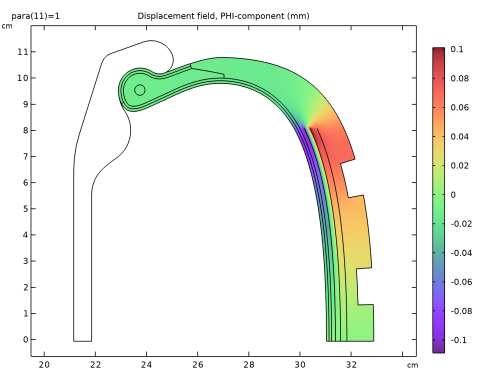
You find the Include circumferential displacement checkbox in the Axial Symmetry Approximation section in the settings window of the Solid Mechanics interface. This allows you to enable the 2D axisymmetric formulation that includes the twist degree of freedom.
|
|
•
|
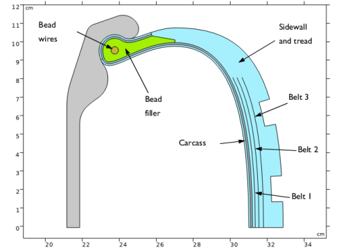
You can add a Initial Stress and Strain node under Linear Elastic Material to model the prestress in the bead wires, resulting after the mounting of the tire on the rim.
|
|
•
|
You can use a Curvilinear Coordinates interface to compute the direction of anisotropy in the carcass.
|
|
•
|
To model the belts without explicitly drawing their thickness, you can simply add a Thin Layer and add a Hyperelastic Material to it. Use the Solid approximation to create a slit for the displacement variable at the selected boundary.
|
|
•
|
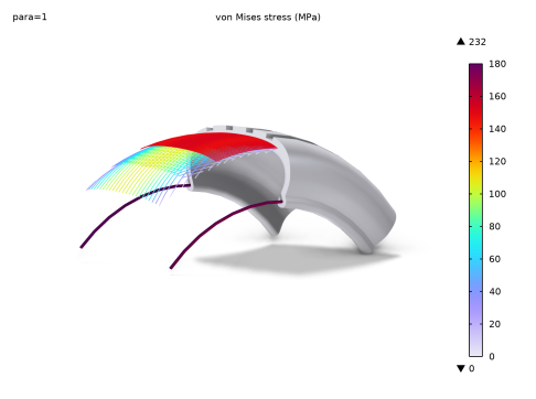
Add three Fiber nodes to the Hyperelastic Material under the Thin Layer in order to model the three different orientations of the cords. You can directly specify the orientation with respect to the boundary coordinate system without further computations. Choose a Linear elastic material model for the cords, to model steel.
|
|
•
|
You find the Antisymmetry option under the Circumferential Condition section when you add the Symmetry Plane.
|
|
1
|
|
2
|
|
3
|
Click Add.
|
|
4
|
Click
|
|
5
|
|
6
|
Click
|
|
1
|
|
2
|
|
1
|
|
2
|
|
3
|
Click
|
|
4
|
Browse to the model’s Application Libraries folder and double-click the file tire_inflation.mphbin.
|
|
5
|
|
1
|
In the Model Builder window, under Global Definitions right-click Geometry Parts and choose 3D Part.
|
|
2
|
|
3
|
|
4
|
|
1
|
|
2
|
Click
|
|
4
|
|
1
|
|
2
|
|
1
|
|
2
|
|
3
|
|
1
|
|
2
|
|
1
|
|
2
|
|
3
|
|
4
|
|
1
|
|
2
|
|
1
|
|
2
|
|
3
|
|
4
|
Click
|
|
1
|
|
2
|
|
3
|
|
1
|
|
2
|
|
3
|
|
4
|
On the object cro1, select Domains 1–3 only.
|
|
5
|
Click
|
|
6
|
|
1
|
|
2
|
On the object pi1, select Point 80 only.
|
|
3
|
|
4
|
|
5
|
|
6
|
|
7
|
Click
|
|
1
|
|
2
|
|
3
|
|
4
|
|
5
|
Select the object ls1 only.
|
|
6
|
Click
|
|
1
|
|
2
|
|
3
|
|
4
|
|
5
|
On the object par1(1), select Domain 1 only.
|
|
6
|
On the object par1(2), select Domains 1, 2, 6, 8, and 10 only.
|
|
7
|
Click
|
|
8
|
|
1
|
|
2
|
|
3
|
Click
|
|
4
|
Browse to the model’s Application Libraries folder and double-click the file tire_inflation_meshcontrol.mphbin.
|
|
5
|
Click to expand the Selections of Resulting Entities section. Select the Resulting objects selection checkbox.
|
|
6
|
|
7
|
Click
|
|
8
|
|
1
|
|
2
|
|
3
|
|
1
|
In the Model Builder window, under 2D Axisymmetric [Tire] (comp1) > Geometry 1 click Form Union (fin).
|
|
2
|
|
3
|
|
4
|
Clear the Create pairs checkbox.
|
|
5
|
Click
|
|
1
|
|
2
|
|
3
|
|
4
|
Click
|
|
5
|
|
1
|
|
2
|
|
4
|
|
5
|
|
6
|
Click to select the
|
|
1
|
In the Model Builder window, under Global Definitions right-click Materials and choose Blank Material.
|
|
2
|
|
3
|
Click to expand the Material Properties section. In the Material properties tree, select Basic Properties > Young’s Modulus.
|
|
4
|
Click
|
|
5
|
|
6
|
Click
|
|
7
|
|
8
|
Click
|
|
9
|
Locate the Material Contents section. In the table, enter the following settings:
|
|
1
|
|
2
|
|
3
|
Locate the Material Contents section. In the table, enter the following settings:
|
|
1
|
|
2
|
|
3
|
Click to expand the Material Properties section. In the Material properties tree, select Solid Mechanics > Hyperelastic Material > Yeoh.
|
|
4
|
Click
|
|
5
|
Locate the Material Contents section. In the table, enter the following settings:
|
|
6
|
Locate the Material Properties section. In the Material properties tree, select Solid Mechanics > Linear Elastic Material > Bulk Modulus and Shear Modulus > Bulk modulus (K).
|
|
7
|
Click
|
|
8
|
Locate the Material Contents section. In the table, enter the following settings:
|
|
9
|
Locate the Material Properties section. In the Material properties tree, select Basic Properties > Density.
|
|
10
|
Click
|
|
11
|
Locate the Material Contents section. In the table, enter the following settings:
|
|
1
|
|
2
|
|
3
|
Locate the Material Contents section. In the table, enter the following settings:
|
|
1
|
|
2
|
|
3
|
Click to expand the Material Properties section. In the Material properties tree, select Solid Mechanics > Linear Elastic Material > Transversely Isotropic.
|
|
4
|
Click
|
|
5
|
|
6
|
Click
|
|
7
|
Locate the Material Contents section. In the table, enter the following settings:
|
|
1
|
In the Model Builder window, under 2D Axisymmetric [Tire] (comp1) right-click Materials and choose More Materials > Material Link.
|
|
2
|
In the Settings window for Material Link, type Material Link: Steel [Bead Wires] in the Label text field.
|
|
3
|
|
5
|
Click
|
|
6
|
|
7
|
Click OK.
|
|
8
|
|
9
|
|
1
|
|
2
|
|
3
|
|
4
|
|
6
|
|
7
|
|
8
|
Click OK.
|
|
9
|
|
10
|
|
11
|
|
1
|
|
2
|
In the Settings window for Material Link, type Material Link: Rubber [Bead] in the Label text field.
|
|
4
|
|
5
|
|
6
|
|
7
|
Click OK.
|
|
8
|
|
9
|
|
10
|
|
1
|
|
2
|
In the Settings window for Material Link, type Material Link: Reinforced Rubber [Carcass] in the Label text field.
|
|
4
|
Locate the Link Settings section. From the Material list, choose Reinforced Rubber [Carcass] (mat5).
|
|
5
|
|
6
|
|
7
|
Click OK.
|
|
8
|
|
9
|
|
1
|
|
2
|
|
3
|
|
4
|
|
5
|
Click OK.
|
|
1
|
|
2
|
|
3
|
|
1
|
|
1
|
|
2
|
|
3
|
|
4
|
|
5
|
|
1
|
|
2
|
In the Settings window for Linear Elastic Material, type Linear Elastic Material [Carcass] in the Label text field.
|
|
3
|
|
4
|
|
5
|
Select the Transversely isotropic checkbox.
|
|
1
|
In the Model Builder window, under 2D Axisymmetric [Tire] (comp1) > Solid Mechanics (solid) click Linear Elastic Material 1.
|
|
2
|
In the Settings window for Linear Elastic Material, type Linear Elastic Material [Bead Wires] in the Label text field.
|
|
1
|
|
2
|
Go to the Add Physics window.
|
|
3
|
|
4
|
Click the Add to 2D Axisymmetric [Tire] button in the window toolbar.
|
|
5
|
|
1
|
|
2
|
|
3
|
|
1
|
|
1
|
|
1
|
In the Model Builder window, under 2D Axisymmetric [Tire] (comp1) > Solid Mechanics (solid) click Linear Elastic Material [Carcass].
|
|
2
|
|
3
|
|
1
|
|
2
|
|
1
|
|
3
|
|
4
|
Click
|
|
5
|
|
6
|
Click OK.
|
|
7
|
|
8
|
|
1
|
|
2
|
|
3
|
|
4
|
|
5
|
|
1
|
In the Model Builder window, under 2D Axisymmetric [Tire] (comp1) > Materials right-click Material Link: Rubber [Sidewall and Tread] (matlnk2) and choose Duplicate.
|
|
2
|
In the Settings window for Material Link, type Material Link: Rubber [Belts] in the Label text field.
|
|
3
|
Locate the Geometric Entity Selection section. From the Geometric entity level list, choose Boundary.
|
|
4
|
|
1
|
|
2
|
|
3
|
|
4
|
|
5
|
|
6
|
Specify the Direction vector as
|
|
7
|
|
8
|
|
9
|
|
11
|
Click
|
|
12
|
|
13
|
Click OK.
|
|
1
|
|
2
|
|
3
|
|
5
|
Click
|
|
6
|
|
7
|
Click OK.
|
|
8
|
|
9
|
Specify the Direction vector as
|
|
1
|
|
2
|
|
3
|
|
5
|
Click
|
|
6
|
|
7
|
Click OK.
|
|
8
|
|
9
|
|
1
|
|
3
|
|
4
|
|
5
|
Select the Include circumferential displacement checkbox.
|
|
1
|
|
2
|
|
3
|
|
1
|
In the Model Builder window, under 2D Axisymmetric [Tire] (comp1) > Solid Mechanics (solid) click Contact 1.
|
|
2
|
|
3
|
|
4
|
|
1
|
|
2
|
|
1
|
|
2
|
|
3
|
|
4
|
Click to expand the Advanced section. Select the Include boundaries external to current physics checkbox.
|
|
5
|
|
6
|
|
8
|
|
1
|
|
2
|
|
3
|
|
1
|
|
2
|
|
4
|
|
5
|
From the list, choose Antisymmetry.
|
|
1
|
|
2
|
|
3
|
|
5
|
Click to expand the Control Entities section. From the Smooth across removed control entities list, choose Off.
|
|
1
|
|
2
|
|
3
|
|
1
|
|
2
|
|
3
|
|
5
|
|
6
|
|
7
|
|
1
|
|
3
|
|
4
|
|
5
|
|
6
|
|
7
|
|
8
|
Select the Reverse direction checkbox.
|
|
1
|
|
3
|
|
4
|
|
5
|
Clear the Reverse direction checkbox.
|
|
1
|
|
3
|
|
4
|
|
1
|
|
3
|
|
4
|
|
1
|
|
3
|
|
4
|
|
1
|
|
2
|
|
3
|
|
4
|
|
1
|
|
3
|
|
4
|
|
1
|
|
2
|
|
3
|
|
4
|
|
5
|
|
6
|
|
7
|
Select the Symmetric distribution checkbox.
|
|
1
|
|
3
|
|
4
|
|
5
|
|
6
|
|
7
|
|
8
|
Click
|
|
1
|
|
2
|
|
3
|
|
5
|
Click
|
|
1
|
|
2
|
|
3
|
|
4
|
Click
|
|
5
|
|
6
|
Click OK.
|
|
7
|
|
8
|
|
1
|
|
3
|
|
4
|
|
1
|
|
2
|
|
3
|
|
1
|
|
1
|
|
2
|
|
3
|
|
1
|
|
2
|
|
3
|
|
1
|
|
3
|
|
4
|
|
5
|
|
6
|
|
7
|
|
8
|
Select the Reverse direction checkbox.
|
|
9
|
Click
|
|
1
|
|
2
|
|
3
|
|
5
|
Locate the Control Entities section. From the Smooth across removed control entities list, choose Off.
|
|
1
|
|
2
|
|
3
|
|
5
|
Click to expand the Control Entities section. From the Smooth across removed control entities list, choose Off.
|
|
1
|
|
2
|
|
3
|
|
1
|
|
2
|
|
3
|
|
4
|
Click
|
|
1
|
|
2
|
|
3
|
|
1
|
|
3
|
|
4
|
|
5
|
Click
|
|
7
|
|
8
|
Click
|
|
1
|
|
2
|
|
3
|
|
4
|
Click the Custom button.
|
|
5
|
Locate the Element Size Parameters section.
|
|
6
|
|
7
|
Click
|
|
1
|
|
2
|
|
3
|
|
4
|
Click
|
|
1
|
|
2
|
In the Geometry Cleanup dialog that opens, click Clean up Automatically to automatically clean up the geometry.
|
|
3
|
|
4
|
|
5
|
|
1
|
|
2
|
|
1
|
|
2
|
|
3
|
Select the Modify model configuration for study step checkbox.
|
|
4
|
|
5
|
Click
|
|
6
|
In the tree, select 2D Axisymmetric [Tire] (comp1) > Solid Mechanics (solid), Controls spatial frame.
|
|
7
|
Click
|
|
8
|
|
1
|
In the Model Builder window, expand the Coordinate system (cc) node, then click Coordinate System Surface 1.
|
|
2
|
|
3
|
|
4
|
|
1
|
|
2
|
Go to the Add Study window.
|
|
3
|
|
4
|
Click the Add Study button in the window toolbar.
|
|
5
|
|
1
|
|
2
|
|
1
|
|
2
|
|
3
|
In the Solve for column of the table, under 2D Axisymmetric [Tire] (comp1), clear the checkbox for Curvilinear Coordinates (cc).
|
|
4
|
Click to expand the Values of Dependent Variables section. Find the Values of variables not solved for subsection. From the Settings list, choose User controlled.
|
|
5
|
|
6
|
|
7
|
|
8
|
Click
|
|
10
|
|
1
|
|
2
|
|
3
|
Click
|
|
4
|
|
5
|
Click OK.
|
|
6
|
|
8
|
Click
|
|
9
|
|
10
|
Click OK.
|
|
11
|
|
13
|
Click
|
|
1
|
|
2
|
Go to the Result Templates window.
|
|
3
|
|
4
|
Click the Add Result Template button in the window toolbar.
|
|
5
|
|
6
|
Click the Add Result Template button in the window toolbar.
|
|
7
|
|
1
|
|
2
|
Select the Show maximum and minimum values checkbox.
|
|
1
|
|
2
|
|
3
|
Select the Manual color range checkbox.
|
|
4
|
|
5
|
|
1
|
|
2
|
In the Settings window for 2D Plot Group, type Out-of-Plane Displacement (solid) in the Label text field.
|
|
1
|
In the Model Builder window, expand the Out-of-Plane Displacement (solid) node, then click Surface 1.
|
|
2
|
|
3
|
|
4
|
|
1
|
|
2
|
|
3
|
|
4
|
|
1
|
|
2
|
In the Settings window for Global, click Replace Expression in the upper-right corner of the y-Axis Data section. From the menu, choose 2D Axisymmetric [Tire] (comp1) > Solid Mechanics > Enclosed cavities > Enclosed Cavity 1 > solid.enc1.V - Total volume, deformed configuration - m³.
|
|
3
|
Locate the y-Axis Data section. In the table, enter the following settings:
|
|
4
|
|
5
|
|
6
|
|
7
|
|
8
|
|
9
|
|
10
|
Select the Only plot when requested checkbox.
|
|
1
|
|
2
|
|
3
|
|
4
|
|
5
|
|
1
|
|
2
|
|
3
|
|
1
|
|
2
|
|
3
|
|
4
|
|
1
|
|
2
|
|
3
|
|
4
|
|
5
|
|
6
|
|
7
|
|
8
|
|
1
|
|
2
|
|
3
|
|
4
|
|
5
|
|
6
|
|
7
|
|
1
|
|
2
|
|
3
|
|
1
|
|
2
|
|
3
|
|
1
|
|
2
|
|
3
|
|
1
|
|
2
|
|
3
|
|
4
|
|
5
|
|
1
|
|
2
|
|
3
|
|
4
|
|
5
|
|
1
|
|
2
|
|
3
|
|
4
|
|
1
|
|
2
|
|
3
|
|
1
|
|
2
|
|
3
|
|
4
|
|
5
|
Locate the Expression section. In the r-component text field, type solid.tl1.hmm1.fibt1.a0R*((mir1side*2)-1).
|
|
6
|
|
7
|
|
9
|
|
10
|
|
11
|
Locate the Coloring and Style section. Find the Line style subsection. From the Type list, choose Tube.
|
|
12
|
|
13
|
|
14
|
|
1
|
|
2
|
|
3
|
|
1
|
|
2
|
|
3
|
|
1
|
|
2
|
|
3
|
|
1
|
|
2
|
|
3
|
|
1
|
|
2
|
|
3
|
|
4
|
Locate the Expression section. In the r-component text field, type solid.tl1.hmm1.fibt2.a0R*((mir1side*2)-1).
|
|
5
|
|
6
|
|
7
|
Locate the Coloring and Style section. Find the Line style subsection. In the Tube radius expression text field, type solid.tl1.hmm1.fibt2.d/2.
|
|
1
|
|
2
|
|
3
|
|
4
|
|
1
|
|
2
|
|
3
|
|
4
|
|
1
|
|
2
|
|
3
|
|
1
|
|
2
|
|
3
|
|
4
|
|
1
|
|
2
|
|
3
|
|
4
|
|
5
|
|
6
|
|
7
|
|
8
|
|
9
|
|
10
|
Locate the Coloring and Style section. Find the Line style subsection. In the Tube radius expression text field, type solid.tl1.hmm1.fibt3.d/2.
|
|
1
|
|
2
|
|
3
|
|
4
|
|
1
|
In the Model Builder window, under Results > Datasets right-click Study: Inflation/Solution 2 (sol2) and choose Duplicate.
|
|
2
|
|
3
|
|
1
|
|
2
|
|
3
|
|
4
|
|
5
|
|
6
|
|
7
|
|
1
|
|
2
|
|
1
|
|
2
|
|
3
|
In the Settings window for 3D Plot Group, type Material and Fiber Direction in the Label text field.
|
|
4
|
|
1
|
|
2
|
|
3
|
|
1
|
|
2
|
|
3
|
|
4
|
|
1
|
|
2
|
|
1
|
|
2
|
|
1
|
|
2
|
|
3
|
Locate the Coloring and Style section. Find the Point style subsection. From the Color list, choose Custom.
|
|
4
|
|
5
|
Click Define custom colors.
|
|
7
|
Click Add to custom colors.
|
|
8
|
|
1
|
|
2
|
|
1
|
|
2
|
|
3
|
Locate the Coloring and Style section. Find the Point style subsection. From the Color list, choose Custom.
|
|
4
|
|
5
|
Click Define custom colors.
|
|
7
|
Click Add to custom colors.
|
|
8
|
|
1
|
|
2
|
|
1
|
|
2
|
|
3
|
Locate the Coloring and Style section. Find the Point style subsection. From the Color list, choose Custom.
|
|
4
|
|
5
|
Click Define custom colors.
|
|
7
|
Click Add to custom colors.
|
|
8
|
|
1
|
|
2
|
|
3
|
|
4
|
|
1
|
|
1
|
|
2
|
|
3
|
|
1
|
|
2
|
|
3
|
|
4
|
Click Replace Expression in the upper-right corner of the Expression section. From the menu, choose 2D Axisymmetric [Tire] (comp1) > Curvilinear Coordinates > cc.e1R,cc.e1PHI,cc.e1Z - First basis vector.
|
|
5
|
|
6
|
|
7
|
|
9
|
|
10
|
Locate the Coloring and Style section. Find the Line style subsection. In the Tube radius expression text field, type dcord_belts/2.
|
|
11
|
|
12
|
|
13
|
Click
|
|
14
|
|
15
|
|
16
|
Clear the Only plot when requested checkbox.
|
|
1
|
|
2
|
|
3
|
|
4
|
In the Settings window for Camera, in the Graphics window toolbar, click
|
|
5
|
|
6
|
|
7
|
|
8
|
|
9
|
|
10
|
|
11
|
|
12
|
|
13
|
|
14
|
|
15
|
|
16
|
|
17
|
|
18
|
|
19
|
|
20
|
|
1
|
|
2
|
|
3
|
|
4
|
|
5
|
|
1
|
|
2
|
|
3
|
Clear the Affected by lighting checkbox.
|
|
4
|
|
5
|
Clear the Casts shadows checkbox.
|
|
6
|
Clear the Receives shadows checkbox.
|
|
7
|
|
8
|
Clear the Casts shadows checkbox.
|
|
9
|
Clear the Receives shadows checkbox.
|
|
10
|
|
1
|
|
2
|
|
1
|
|
2
|
|
3
|
|
4
|