PDF

Thin Layer Interfaces
Introduction
This model demonstrates alternative implementations for describing a thin layer, and the impact of the choice on the continuity of the displacement and stress fields. It is shown how a perfect interface can be obtained by asymptotically changing the material parameters.
Model Definition
Figure 1 shows the undeformed geometry composed by two domains forming a square of side L and the contacting surface where the thin layer interface will be placed. The full domain is a square of side 1 m and the interface is built by joining two circular arcs of radius 0.707.
Figure 1: Model geometry.
A nearly incompressible Saint-Venant–Kirchhoff hyperelastic material is used for both domains. The thin layer of thickness d << L contains a compressible Saint-Venant–Kirchhoff hyperelastic material. The domain material properties are shown in Table 1.
thin layer approximations
This study uses three approximations:
In the solid approximation, a slit is introduced and consequently a discontinuity of the displacement field is allowed. The slit is filled with a 3D thin material whose deformation gradient, F, is approximated as
(1)
Here, ue is the extension of the layer, ua is the average displacement of the layer mid-plane, and N is the normal.
In the membrane approximation, no slit is introduced; the continuity of the displacement is assured and only a jump in the stress is permitted. The deformation gradient is approximated as follows:
(2)
The material properties for both the solid and membrane approximations are given in terms of the bulk modulus kb and the shear modulus μb.
If a spring material is used, a slit is introduced as in the solid case and the two sides of the interface are connected by springs. The deformation gradient is approximated as
(3)
and the resulting geometric nonlinear spring force fs per unit area is defined as
(4)
where α is the spring stiffness constant.
Boundary conditions
A prescribed displacement boundary condition is applied on the lateral faces in the normal direction up to a stretch of 50%. The upper and lower faces are constrained with a roller.
Results and Discussion
In the case of a perfect interface, the displacement and stresses are continuous, as shown in Figure 2.
Figure 2: First Piola–Kirchhoff stress (xX component) for the perfect interface case after a 50% stretch. Continuity of displacements and stresses along the interface are enforced.
If a thin layer of material is inserted between the domains, the perfect continuity of the stress and displacements is no longer ensured. For example, when using a solid approximation, both the stress and displacement fields are discontinuous, as shown in Figure 3.
Figure 3: First Piola–Kirchhoff stress distribution with a thin layer using a solid approximation.
The displacement can be enforced to be continuous using the membrane approximation. Moreover, if the ratio between the shear modulus of the thin layer and the bulk material goes to zero, the continuity of the stress is also restored.
Figure 4: First Piola–Kirchhoff stress distribution with a thin layer using the membrane approximation.
Figure 5: Stress at the center point. Comparison between thin layer (membrane approximation) and perfect interface.
If a spring material is used, the displacements are no more continuous but the stresses are. If the stiffness of the spring increases, the displacement jump disappears resulting in a perfect interface.
Figure 6: First Piola–Kirchhoff stress distribution with a thin layer using a spring material.
Figure 7: Stress at the center point. Comparison between thin layer (spring material) and perfect interface.
Reference
1. A. Javili, “Variational formulation of generalized interfaces for finite deformation elasticity,” Math. Mech. Solids, vol. 23, 2018.
Application Library path: Nonlinear_Structural_Materials_Module/Hyperelasticity/thin_layer_interfaces
Modeling Instructions
From the File menu, choose New.
New
In the New window, click  Model Wizard.
Model Wizard
1
In the Model Wizard window, click  2D.
2
In the Select Physics tree, select Structural Mechanics > Solid Mechanics (solid).
3
Click Add.
4
Click  Study.
5
Global Definitions
Parameters 1
1
In the Model Builder window, under Global Definitions click Parameters 1.
2
In the Settings window for Parameters, locate the Parameters section.
3
Click  Load from File.
4
Geometry 1
Square 1 (sq1)
1
In the Model Builder window, expand the Component 1 (comp1) > Geometry 1 node.
2
Right-click Geometry 1 and choose Square.
3
In the Settings window for Square, locate the Size section.
4
In the Side length text field, type L.
Circular Arc 1 (ca1)
1
In the Geometry toolbar, click  More Primitives and choose Circular Arc.
2
In the Settings window for Circular Arc, locate the Radius section.
3
In the Radius text field, type R.
4
Locate the Angles section. In the End angle text field, type 45.
Circular Arc 2 (ca2)
1
Right-click Circular Arc 1 (ca1) and choose Duplicate.
2
In the Settings window for Circular Arc, locate the Center section.
3
In the x text field, type L.
4
In the y text field, type L.
5
Locate the Angles section. In the Start angle text field, type 180.
6
In the End angle text field, type 225.
Partition Objects 1 (par1)
1
In the Geometry toolbar, click  Booleans and Partitions and choose Partition Objects.
2
3
In the Settings window for Partition Objects, locate the Partition Objects section.
4
Click to select the  Activate Selection toggle button for Tool objects.
5
Select the objects ca1 and ca2 only.
Form Union (fin)
1
In the Home toolbar, click  Build All.
2
Click the  Zoom Extents button in the Graphics toolbar.
Add an average operator for plotting purposes.
Definitions
Average 1 (aveop1)
1
In the Definitions toolbar, click  Nonlocal Couplings and choose Average.
2
Click in the Graphics window and then press Ctrl+A to select both domains.
Solid Mechanics (solid)
1
In the Model Builder window, under Component 1 (comp1) click Solid Mechanics (solid).
2
In the Settings window for Solid Mechanics, locate the Thickness section.
3
In the d text field, type d.
Hyperelastic Material 1
1
In the Physics toolbar, click  Domains and choose Hyperelastic Material.
2
Click in the Graphics window and then press Ctrl+A to select both domains.
3
In the Settings window for Hyperelastic Material, locate the Hyperelastic Material section.
4
From the Material model list, choose Saint-Venant–Kirchhoff.
5
From the Specify list, choose Bulk modulus and shear modulus.
6
From the Compressibility list, choose Nearly incompressible.
Materials
Bulk
1
In the Model Builder window, under Component 1 (comp1) right-click Materials and choose Blank Material.
2
In the Settings window for Material, type Bulk in the Label text field.
3
Locate the Material Contents section. In the table, enter the following settings:
Solid Mechanics (solid)
Roller 1
1
In the Physics toolbar, click  Boundaries and choose Roller.
2
Prescribed Displacement 1
1
In the Physics toolbar, click  Boundaries and choose Prescribed Displacement.
2
3
In the Settings window for Prescribed Displacement, locate the Coordinate System Selection section.
4
From the Coordinate system list, choose Boundary System 1 (sys1).
5
Locate the Prescribed Displacement section. From the Displacement in t1 direction list, choose Prescribed.
6
From the Displacement in n direction list, choose Prescribed.
7
In the u0n text field, type L*stretch/2.
Mesh 1
Mapped 1
In the Mesh toolbar, click  Mapped.
Distribution 1
1
Right-click Mapped 1 and choose Distribution.
2
3
In the Settings window for Distribution, locate the Distribution section.
4
In the Number of elements text field, type nel.
Distribution 2
1
In the Model Builder window, right-click Mapped 1 and choose Distribution.
2
In the Settings window for Distribution, locate the Distribution section.
3
From the Distribution type list, choose Predefined.
4
5
In the Number of elements text field, type nel.
6
In the Element ratio text field, type 3.
Distribution 3
1
Right-click Distribution 2 and choose Duplicate.
2
Distribution 4
1
In the Model Builder window, right-click Mapped 1 and choose Distribution.
2
3
In the Settings window for Distribution, locate the Distribution section.
4
In the Number of elements text field, type nel*2.
5
Click  Build All.
Add Study
1
In the Home toolbar, click  Add Study to open the Add Study window.
2
Go to the Add Study window.
3
Find the Studies subsection. In the Select Study tree, select General Studies > Stationary.
4
Click the Add Study button in the window toolbar.
5
In the Home toolbar, click  Add Study to close the Add Study window.
Perfect Interface
1
In the Settings window for Study, type Perfect Interface in the Label text field.
2
Locate the Study Settings section. Clear the Generate default plots checkbox.
Step 1: Stationary
1
In the Model Builder window, under Perfect Interface click Step 1: Stationary.
2
In the Settings window for Stationary, click to expand the Study Extensions section.
3
Select the Auxiliary sweep checkbox.
4
5
6
Click  Range.
7
In the Range dialog, type 0.1 in the Start text field.
8
In the Step text field, type 0.1.
9
In the Stop text field, type 0.5.
10
Click Replace.
11
In the Study toolbar, click  Compute.
Set default units for result presentation.
Results
Preferred Units 1
1
In the Model Builder window, expand the Results node.
2
Right-click Results and choose Preferred Units.
3
In the Settings window for Preferred Units, locate the Units section.
4
Click  Add Physical Quantity.
5
In the Physical Quantity dialog, select Solid Mechanics > Stress tensor (N/m^2) in the tree.
6
7
In the Settings window for Preferred Units, locate the Units section.
8
9
Select the Apply conversions to expressions with the same dimensions checkbox.
10
Click  Apply.
Perfect Interface
1
In the Results toolbar, click  2D Plot Group.
2
In the Settings window for 2D Plot Group, type Perfect Interface in the Label text field.
3
Click to expand the Title section. From the Title type list, choose Manual.
4
In the Title text area, type Perfect Interface.
5
Clear the Parameter indicator text field.
Surface 1
1
Right-click Perfect Interface and choose Surface.
2
In the Settings window for Surface, locate the Expression section.
3
In the Expression text field, type solid.PxX.
Deformation 1
1
Right-click Surface 1 and choose Deformation.
2
In the Settings window for Deformation, locate the Scale section.
3
Select the Scale factor checkbox. In the associated text field, type 1.
Perfect Interface
1
In the Model Builder window, under Results click Perfect Interface.
2
In the Settings window for 2D Plot Group, locate the Plot Settings section.
3
From the View list, choose New view.
4
In the Perfect Interface toolbar, click  Plot.
5
Click the  Zoom Extents button in the Graphics toolbar.
Add a thin layer between the domains using a solid approximation.
Solid Mechanics (solid)
Solid Approximation
1
In the Physics toolbar, click  Boundaries and choose Thin Layer.
2
3
In the Settings window for Thin Layer, locate the Boundary Properties section.
4
In the Lth text field, type th.
5
In the Label text field, type Solid Approximation.
Hyperelastic Material 1
1
In the Physics toolbar, click  Attributes and choose Hyperelastic Material.
2
3
In the Settings window for Hyperelastic Material, locate the Hyperelastic Material section.
4
From the Material model list, choose Saint-Venant–Kirchhoff.
5
From the Specify list, choose Bulk modulus and shear modulus.
Materials
Thin Layer
1
In the Model Builder window, under Component 1 (comp1) right-click Materials and choose Blank Material.
2
In the Settings window for Material, type Thin Layer in the Label text field.
3
Locate the Geometric Entity Selection section. From the Geometric entity level list, choose Boundary.
4
5
Locate the Material Contents section. In the table, enter the following settings:
Add Study
1
In the Home toolbar, click  Add Study to open the Add Study window.
2
Go to the Add Study window.
3
Find the Studies subsection. In the Select Study tree, select General Studies > Stationary.
4
Click the Add Study button in the window toolbar.
5
In the Home toolbar, click  Add Study to close the Add Study window.
Study 2
Step 1: Stationary
1
In the Settings window for Stationary, locate the Study Extensions section.
2
Select the Auxiliary sweep checkbox.
3
4
5
6
7
From the Sweep type list, choose All combinations.
8
From the Run continuation for list, choose Manual.
9
From the Continuation parameter list, choose stretch.
10
In the Model Builder window, click Study 2.
11
In the Settings window for Study, locate the Study Settings section.
12
Clear the Generate default plots checkbox.
13
In the Label text field, type Solid Approximation.
14
In the Study toolbar, click  Compute.
Results
Solid Approximation
1
In the Results toolbar, click  2D Plot Group.
2
In the Settings window for 2D Plot Group, type Solid Approximation in the Label text field.
3
Locate the Data section. From the Dataset list, choose Solid Approximation/Solution 2 (sol2).
4
Locate the Title section. From the Title type list, choose Manual.
5
In the Title text area, type Thin Layer Using Solid Thickness Approximation.
6
Clear the Parameter indicator text field.
Surface 1
1
Right-click Solid Approximation and choose Surface.
2
In the Settings window for Surface, locate the Expression section.
3
In the Expression text field, type solid.PxX.
4
In the Solid Approximation toolbar, click  Plot.
Deformation 1
1
Right-click Surface 1 and choose Deformation.
2
In the Settings window for Deformation, locate the Scale section.
3
Select the Scale factor checkbox. In the associated text field, type 1.
Solid Approximation
1
In the Model Builder window, under Results click Solid Approximation.
2
In the Settings window for 2D Plot Group, locate the Data section.
3
From the Parameter value (MuRatio) list, choose 0.25.
4
In the Solid Approximation toolbar, click  Plot.
Arrow Line 1
Right-click Solid Approximation and choose Arrow Line.
Deformation 1
1
In the Model Builder window, right-click Arrow Line 1 and choose Deformation.
2
In the Settings window for Deformation, locate the Scale section.
3
Select the Scale factor checkbox. In the associated text field, type 1.
4
In the Solid Approximation toolbar, click  Plot.
Arrow Line 1
1
In the Model Builder window, click Arrow Line 1.
2
In the Settings window for Arrow Line, locate the Arrow Positioning section.
3
From the Placement list, choose Mesh vertices.
4
Click Replace Expression in the upper-right corner of the Expression section. From the menu, choose Component 1 (comp1) > Solid Mechanics > Displacement > u,v - Displacement field.
Selection 1
1
Right-click Arrow Line 1 and choose Selection.
2
Solid Approximation
1
In the Model Builder window, under Results click Solid Approximation.
2
In the Settings window for 2D Plot Group, locate the Plot Settings section.
3
From the View list, choose View 2D 2.
4
In the Solid Approximation toolbar, click  Plot.
Add a thin layer using a membrane approximation to get an elastic interface model.
Solid Mechanics (solid)
Membrane Approximation
1
In the Physics toolbar, click  Boundaries and choose Thin Layer.
2
In the Settings window for Thin Layer, type Membrane Approximation in the Label text field.
3
4
Locate the Boundary Properties section. In the Lth text field, type th.
5
Locate the Thin Layer section. From the Approximation list, choose Membrane.
Hyperelastic Material 1
1
In the Physics toolbar, click  Attributes and choose Hyperelastic Material.
2
3
In the Settings window for Hyperelastic Material, locate the Hyperelastic Material section.
4
From the Material model list, choose Saint-Venant–Kirchhoff.
5
From the Specify list, choose Bulk modulus and shear modulus.
Add Study
1
In the Home toolbar, click  Add Study to open the Add Study window.
2
Go to the Add Study window.
3
Find the Studies subsection. In the Select Study tree, select General Studies > Stationary.
4
Click the Add Study button in the window toolbar.
5
In the Home toolbar, click  Add Study to close the Add Study window.
Membrane Approximation
1
In the Settings window for Study, type Membrane Approximation in the Label text field.
2
Locate the Study Settings section. Clear the Generate default plots checkbox.
Step 1: Stationary
1
In the Model Builder window, under Membrane Approximation click Step 1: Stationary.
2
In the Settings window for Stationary, locate the Physics and Variables Selection section.
3
Select the Modify model configuration for study step checkbox.
4
In the tree, select Component 1 (comp1) > Solid Mechanics (solid), Controls spatial frame > Solid Approximation.
5
Click  Disable.
6
Locate the Study Extensions section. Select the Auxiliary sweep checkbox.
7
8
9
Click  Range.
10
In the Range dialog, type 0.1 in the Start text field.
11
In the Step text field, type 0.1.
12
In the Stop text field, type 0.5.
13
Click Add.
14
In the Settings window for Stationary, locate the Study Extensions section.
15
16
17
From the Sweep type list, choose All combinations.
18
From the Run continuation for list, choose Manual.
19
From the Continuation parameter list, choose stretch.
20
In the Study toolbar, click  Compute.
Results
Membrane Approximation
1
In the Results toolbar, click  2D Plot Group.
2
In the Settings window for 2D Plot Group, type Membrane Approximation in the Label text field.
3
Locate the Data section. From the Dataset list, choose Membrane Approximation/Solution 3 (sol3).
4
Locate the Title section. From the Title type list, choose Manual.
5
In the Title text area, type Transition from Membrane Approximation to Perfect Interface.
6
Clear the Parameter indicator text field.
7
Click to expand the Plot Array section. From the Array type list, choose Square.
8
From the Padding list, choose Absolute.
9
In the Column padding length text field, type L.
10
In the Row padding length text field, type -2.4*L.
Surface 1
1
Right-click Membrane Approximation and choose Surface.
2
In the Settings window for Surface, locate the Data section.
3
From the Dataset list, choose Membrane Approximation/Solution 3 (sol3).
4
Locate the Expression section. In the Expression text field, type solid.PxX.
Deformation 1
1
Right-click Surface 1 and choose Deformation.
2
In the Settings window for Deformation, locate the Scale section.
3
Select the Scale factor checkbox. In the associated text field, type 1.
4
In the Membrane Approximation toolbar, click  Plot.
Solution Array 1
1
In the Model Builder window, right-click Surface 1 and choose Solution Array.
2
In the Settings window for Solution Array, locate the Data section.
3
From the Parameter selection (stretch) list, choose Last.
4
From the Parameter selection (MuRatio) list, choose Manual.
5
In the Parameter indices (1-8) text field, type 8 7 6 4 3.
6
Locate the Plot Array section. From the Array shape list, choose Square.
Surface 2
1
In the Model Builder window, right-click Membrane Approximation and choose Surface.
2
In the Settings window for Surface, locate the Data section.
3
From the Dataset list, choose Perfect Interface/Solution 1 (sol1).
4
Locate the Expression section. In the Expression text field, type solid.PxX.
5
Click to expand the Inherit Style section. From the Plot list, choose Surface 1.
6
Click to expand the Plot Array section. Select the Manual indexing checkbox.
7
In the Column index text field, type 2.
8
In the Row index text field, type 1.
Deformation 1
Right-click Surface 2 and choose Deformation.
Table Annotation 1
1
In the Membrane Approximation toolbar, click  More Plots and choose Table Annotation.
2
In the Settings window for Table Annotation, locate the Data section.
3
From the Source list, choose Local table.
4
5
Locate the Coloring and Style section. Clear the Show point checkbox.
6
Locate the Data section. Select the LaTeX markup checkbox.
Membrane Approximation
1
In the Model Builder window, click Membrane Approximation.
2
In the Settings window for 2D Plot Group, locate the Plot Settings section.
3
From the View list, choose New view.
4
In the Membrane Approximation toolbar, click  Plot.
Line Plot: Membrane Approximation
1
In the Results toolbar, click  1D Plot Group.
2
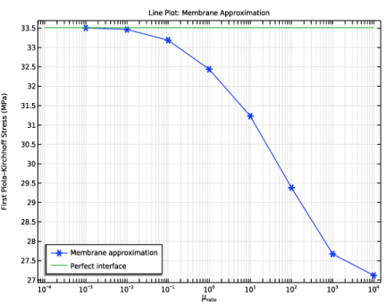
In the Settings window for 1D Plot Group, type Line Plot: Membrane Approximation in the Label text field.
3
Locate the Data section. From the Dataset list, choose Membrane Approximation/Solution 3 (sol3).
4
Locate the Axis section. Select the x-axis log scale checkbox.
5
Locate the Plot Settings section.
6
Select the x-axis label checkbox. In the associated text field, type \mu<sub>ratio</sub>.
7
Select the y-axis label checkbox. In the associated text field, type First Piola-Kirchhoff Stress (MPa).
8
Click to expand the Title section. From the Title type list, choose Label.
9
Locate the Legend section. From the Position list, choose Lower left.
Point Graph 1
1
Right-click Line Plot: Membrane Approximation and choose Point Graph.
2
3
In the Settings window for Point Graph, locate the y-Axis Data section.
4
In the Expression text field, type mean(side(1,solid.PxX)).
5
Locate the x-Axis Data section. From the Axis source data list, choose MuRatio.
6
Locate the Data section. From the Dataset list, choose Membrane Approximation/Solution 3 (sol3).
7
From the Parameter selection (stretch) list, choose Last.
8
Click to expand the Legends section. Select the Show legends checkbox.
9
From the Legends list, choose Manual.
10
11
Click to expand the Coloring and Style section. Find the Line markers subsection. From the Marker list, choose Cycle.
12
In the Line Plot: Membrane Approximation toolbar, click  Plot.
Line Segments 1
1
In the Model Builder window, right-click Line Plot: Membrane Approximation and choose Line Segments.
2
In the Settings window for Line Segments, locate the Data section.
3
From the Dataset list, choose Perfect Interface/Solution 1 (sol1).
4
From the Parameter selection (stretch) list, choose Last.
5
Locate the x-Coordinates section. In the table, enter the following settings:
6
Locate the y-Coordinates section. In the table, enter the following settings:
7
Click to expand the Legends section. Select the Show legends checkbox.
8
From the Legends list, choose Manual.
9
10
Click the  Zoom Extents button in the Graphics toolbar.
Add a thin layer using a spring approximation to mimic a cohesive interface model.
Solid Mechanics (solid)
Spring Approximation
1
In the Physics toolbar, click  Boundaries and choose Thin Layer.
2
3
In the Settings window for Thin Layer, locate the Boundary Properties section.
4
In the Lth text field, type th.
5
Locate the Thin Layer section. From the Approximation list, choose Spring.
6
In the Label text field, type Spring Approximation.
Spring Material 1
1
In the Physics toolbar, click  Attributes and choose Spring Material.
2
In the Settings window for Spring Material, locate the Spring section.
3
In the kA text field, type AlphaBnd.
4
In the ρV text field, type RhoBnd.
5
Add Study
1
In the Home toolbar, click  Add Study to open the Add Study window.
2
Go to the Add Study window.
3
Find the Studies subsection. In the Select Study tree, select General Studies > Stationary.
4
Click the Add Study button in the window toolbar.
5
In the Home toolbar, click  Add Study to close the Add Study window.
Spring Approximation
1
In the Settings window for Study, type Spring Approximation in the Label text field.
2
Locate the Study Settings section. Clear the Generate default plots checkbox.
Step 1: Stationary
1
In the Model Builder window, under Spring Approximation click Step 1: Stationary.
2
In the Settings window for Stationary, locate the Physics and Variables Selection section.
3
Select the Modify model configuration for study step checkbox.
4
In the tree, select Component 1 (comp1) > Solid Mechanics (solid), Controls spatial frame > Solid Approximation and Component 1 (comp1) > Solid Mechanics (solid), Controls spatial frame > Membrane Approximation.
5
Click  Disable.
6
Locate the Study Extensions section. Select the Auxiliary sweep checkbox.
7
8
9
10
11
From the Sweep type list, choose All combinations.
12
From the Run continuation for list, choose Manual.
13
From the Continuation parameter list, choose stretch.
14
In the Study toolbar, click  Compute.
Results
Spring Approximation
1
In the Results toolbar, click  2D Plot Group.
2
In the Settings window for 2D Plot Group, type Spring Approximation in the Label text field.
3
Locate the Data section. From the Dataset list, choose Spring Approximation/Solution 4 (sol4).
4
Locate the Title section. From the Title type list, choose Manual.
5
In the Title text area, type Transition from Spring Approximation to Perfect Interface.
6
Clear the Parameter indicator text field.
7
Locate the Plot Settings section. From the View list, choose View 2D 3.
8
Locate the Plot Array section. From the Array type list, choose Square.
9
From the Padding list, choose Absolute.
10
In the Column padding length text field, type L.
11
In the Row padding length text field, type -2.4*L.
Surface 1
1
Right-click Spring Approximation and choose Surface.
2
In the Settings window for Surface, locate the Data section.
3
From the Dataset list, choose Spring Approximation/Solution 4 (sol4).
4
From the Parameter value (AlphaRatio) list, choose 0.001.
5
Locate the Expression section. In the Expression text field, type solid.PxX.
Deformation 1
1
Right-click Surface 1 and choose Deformation.
2
In the Settings window for Deformation, locate the Scale section.
3
Select the Scale factor checkbox. In the associated text field, type 1.
4
In the Spring Approximation toolbar, click  Plot.
Solution Array 1
1
In the Model Builder window, right-click Surface 1 and choose Solution Array.
2
In the Settings window for Solution Array, locate the Data section.
3
From the Parameter selection (stretch) list, choose Last.
4
From the Parameter selection (AlphaRatio) list, choose From list.
5
In the Parameter values (AlphaRatio) list, choose 0.001, 0.1, 1, 10, and 1000.
6
Locate the Plot Array section. From the Array shape list, choose Square.
Surface 2
1
In the Model Builder window, right-click Spring Approximation and choose Surface.
2
In the Settings window for Surface, locate the Data section.
3
From the Dataset list, choose Perfect Interface/Solution 1 (sol1).
4
Locate the Expression section. In the Expression text field, type solid.PxX.
5
Locate the Inherit Style section. From the Plot list, choose Surface 1.
6
Locate the Plot Array section. Select the Manual indexing checkbox.
7
In the Column index text field, type 2.
8
In the Row index text field, type 1.
Deformation 1
Right-click Surface 2 and choose Deformation.
Table Annotation 1
1
In the Spring Approximation toolbar, click  More Plots and choose Table Annotation.
2
In the Settings window for Table Annotation, locate the Data section.
3
From the Source list, choose Local table.
4
5
Locate the Coloring and Style section. Clear the Show point checkbox.
6
Locate the Data section. Select the LaTeX markup checkbox.
7
In the Spring Approximation toolbar, click  Plot.
8
Click the  Zoom Extents button in the Graphics toolbar.
Line Plot: Spring Approximation
1
In the Model Builder window, right-click Line Plot: Membrane Approximation and choose Duplicate.
2
In the Settings window for 1D Plot Group, locate the Data section.
3
From the Dataset list, choose Spring Approximation/Solution 4 (sol4).
4
Locate the Plot Settings section. In the x-axis label text field, type \alpha<sub>ratio</sub>.
5
In the Label text field, type Line Plot: Spring Approximation.
6
Locate the Legend section. From the Position list, choose Lower right.
Point Graph 1
1
In the Model Builder window, expand the Line Plot: Spring Approximation node, then click Point Graph 1.
2
In the Settings window for Point Graph, locate the Data section.
3
From the Dataset list, choose Spring Approximation/Solution 4 (sol4).
4
Locate the Legends section. In the table, enter the following settings:
5
In the Line Plot: Spring Approximation toolbar, click  Plot.
Line Segments 1
1
In the Model Builder window, click Line Segments 1.
2
In the Settings window for Line Segments, locate the x-Coordinates section.
3
4
In the Line Plot: Spring Approximation toolbar, click  Plot.
Disable some features in the studies to be able to rerun them.
Perfect Interface
Step 1: Stationary
1
In the Model Builder window, under Perfect Interface click Step 1: Stationary.
2
In the Settings window for Stationary, locate the Physics and Variables Selection section.
3
Select the Modify model configuration for study step checkbox.
4
In the tree, select Component 1 (comp1) > Solid Mechanics (solid), Controls spatial frame > Solid Approximation, Component 1 (comp1) > Solid Mechanics (solid), Controls spatial frame > Membrane Approximation, and Component 1 (comp1) > Solid Mechanics (solid), Controls spatial frame > Spring Approximation.
5
Click  Disable.
Solid Approximation
1
In the Model Builder window, under Solid Approximation click Step 1: Stationary.
2
In the Settings window for Stationary, locate the Physics and Variables Selection section.
3
Select the Modify model configuration for study step checkbox.
4
In the tree, select Component 1 (comp1) > Solid Mechanics (solid), Controls spatial frame > Membrane Approximation and Component 1 (comp1) > Solid Mechanics (solid), Controls spatial frame > Spring Approximation.
5
Click  Disable.
Membrane Approximation
1
In the Model Builder window, under Membrane Approximation click Step 1: Stationary.
2
In the Settings window for Stationary, locate the Physics and Variables Selection section.
3
In the tree, select Component 1 (comp1) > Solid Mechanics (solid), Controls spatial frame > Spring Approximation.
4
Click  Disable.