|
|
|
|
•
|
|
•
|
|
•
|
|
•
|
|
α (1/°C)
|
16·10-6
|
16.5·10-6
|
17·10-6
|
17.5·10-6
|
|
cp (J/(kg·K))
|
||||
|
σys(0.0) (MPa)
|
||||
|
σys(0.0004) (MPa)
|
||||
|
σys(0.001) (MPa)
|
||||
|
σys(0.002) (MPa)
|
||||
|
σys(0.004) (MPa)
|
||||
|
σys(0.001) (MPa)
|
|
α (1/°C)
|
10.910-6
|
12.410-6
|
13.810-6
|
14.910-6
|
|
cp (J/(kg·K))
|
||||
|
1
|
|
2
|
In the Select Physics tree, select Structural Mechanics > Thermal–Structure Interaction > Thermal Stress, Solid.
|
|
3
|
Click Add.
|
|
4
|
Click
|
|
5
|
|
6
|
Click
|
|
1
|
|
2
|
|
1
|
|
2
|
Browse to the model’s Application Libraries folder and double-click the file temperature_dependent_plasticity_geom_sequence.mph.
|
|
3
|
|
4
|
|
5
|
|
1
|
|
3
|
|
4
|
|
1
|
In the Model Builder window, under Component 1 (comp1) right-click Materials and choose Blank Material.
|
|
2
|
|
4
|
Locate the Material Contents section. In the table, enter the following settings:
|
|
1
|
In the Model Builder window, expand the Component 1 (comp1) > Materials > Stainless Steel (mat1) node.
|
|
2
|
Right-click Component 1 (comp1) > Materials > Stainless Steel (mat1) > Young’s modulus and Poisson’s ratio (Enu) and choose Functions > Interpolation.
|
|
3
|
|
4
|
|
6
|
|
7
|
In the Function table, enter the following settings:
|
|
1
|
In the Model Builder window, under Component 1 (comp1) > Materials > Stainless Steel (mat1) click Young’s modulus and Poisson’s ratio (Enu).
|
|
2
|
|
3
|
Click
|
|
4
|
|
5
|
|
6
|
Click OK.
|
|
7
|
In the Settings window for Young’s Modulus and Poisson’s Ratio, locate the Output Properties section.
|
|
1
|
|
2
|
|
3
|
|
5
|
|
6
|
In the Function table, enter the following settings:
|
|
1
|
|
2
|
|
3
|
|
5
|
|
6
|
In the Function table, enter the following settings:
|
|
1
|
|
2
|
|
3
|
|
5
|
|
6
|
In the Function table, enter the following settings:
|
|
1
|
In the Model Builder window, under Component 1 (comp1) > Materials > Stainless Steel (mat1) click Basic (def).
|
|
2
|
|
3
|
Click
|
|
4
|
|
5
|
|
6
|
Click OK.
|
|
7
|
|
8
|
|
10
|
Click to expand the Material Properties section. In the Material properties tree, select Solid Mechanics > Elastoplastic Material > Elastoplastic Material Model.
|
|
11
|
Click
|
|
1
|
|
2
|
|
3
|
|
4
|
Click
|
|
5
|
Browse to the model’s Application Libraries folder and double-click the file temperature_dependent_plasticity_function.txt.
|
|
6
|
Locate the Data Column Settings section. In the table, click to select the cell at row number 1 and column number 1.
|
|
7
|
|
9
|
|
11
|
|
12
|
|
13
|
|
1
|
In the Model Builder window, under Component 1 (comp1) > Materials > Stainless Steel (mat1) click Elastoplastic material model (ElastoplasticModel).
|
|
2
|
|
3
|
Click
|
|
4
|
|
5
|
|
6
|
Click OK.
|
|
7
|
|
8
|
Click
|
|
9
|
|
10
|
|
11
|
Click OK.
|
|
12
|
|
1
|
|
2
|
|
4
|
Locate the Material Contents section. In the table, enter the following settings:
|
|
1
|
|
2
|
Right-click Component 1 (comp1) > Materials > Carbon Steel (mat2) > Young’s modulus and Poisson’s ratio (Enu) and choose Functions > Interpolation.
|
|
3
|
|
4
|
|
6
|
|
7
|
In the Function table, enter the following settings:
|
|
1
|
In the Model Builder window, under Component 1 (comp1) > Materials > Carbon Steel (mat2) click Young’s modulus and Poisson’s ratio (Enu).
|
|
2
|
|
3
|
Click
|
|
4
|
|
5
|
|
6
|
Click OK.
|
|
1
|
|
2
|
|
3
|
|
5
|
|
6
|
In the Function table, enter the following settings:
|
|
1
|
|
2
|
|
3
|
|
5
|
|
6
|
In the Function table, enter the following settings:
|
|
1
|
|
2
|
|
3
|
|
5
|
|
6
|
In the Function table, enter the following settings:
|
|
1
|
In the Model Builder window, under Component 1 (comp1) > Materials > Carbon Steel (mat2) click Basic (def).
|
|
2
|
|
3
|
Click
|
|
4
|
|
5
|
|
6
|
Click OK.
|
|
7
|
|
8
|
|
1
|
|
2
|
|
3
|
|
4
|
|
5
|
|
1
|
|
2
|
|
3
|
|
5
|
|
6
|
In the Function table, enter the following settings:
|
|
1
|
|
2
|
|
3
|
|
1
|
In the Model Builder window, under Component 1 (comp1) > Heat Transfer in Solids (ht) click Initial Values 1.
|
|
2
|
|
3
|
|
1
|
|
2
|
|
3
|
|
1
|
|
3
|
|
4
|
|
5
|
|
6
|
|
1
|
|
3
|
|
4
|
|
5
|
|
6
|
|
1
|
|
3
|
|
4
|
|
5
|
|
6
|
|
1
|
|
2
|
|
3
|
|
1
|
|
3
|
|
4
|
From the list, choose Free displacement.
|
|
1
|
|
3
|
|
4
|
From the list, choose Free displacement.
|
|
1
|
|
3
|
|
4
|
|
5
|
|
1
|
|
3
|
|
4
|
|
1
|
|
2
|
|
3
|
|
4
|
|
6
|
|
1
|
|
1
|
|
2
|
|
3
|
Click the Custom button.
|
|
4
|
Locate the Element Size Parameters section.
|
|
5
|
|
1
|
|
2
|
|
3
|
|
1
|
|
1
|
|
2
|
|
3
|
Click the Custom button.
|
|
4
|
Locate the Element Size Parameters section.
|
|
5
|
|
1
|
|
2
|
|
3
|
|
1
|
|
2
|
|
3
|
|
4
|
|
5
|
Select the Reverse direction checkbox.
|
|
1
|
|
2
|
|
3
|
|
1
|
|
2
|
|
3
|
|
1
|
|
2
|
|
3
|
|
4
|
Click
|
|
1
|
|
2
|
|
3
|
|
4
|
|
1
|
|
2
|
Go to the Add Study window.
|
|
3
|
|
4
|
Find the Physics interfaces in study subsection. In the table, clear the Solve checkbox for Solid Mechanics (solid).
|
|
5
|
Click the Add Study button in the window toolbar.
|
|
1
|
|
2
|
|
3
|
Click to expand the Values of Dependent Variables section. Find the Initial values of variables solved for subsection. From the Settings list, choose User controlled.
|
|
4
|
|
5
|
|
6
|
Find the Values of variables not solved for subsection. From the Settings list, choose User controlled.
|
|
7
|
|
8
|
|
9
|
|
10
|
|
11
|
|
1
|
|
2
|
|
3
|
|
4
|
|
5
|
|
1
|
Go to the Add Study window.
|
|
2
|
|
3
|
Find the Physics interfaces in study subsection. In the table, clear the Solve checkbox for Heat Transfer in Solids (ht).
|
|
4
|
Click the Add Study button in the window toolbar.
|
|
5
|
|
1
|
|
2
|
Find the Initial values of variables solved for subsection. From the Settings list, choose User controlled.
|
|
3
|
|
4
|
|
5
|
Find the Values of variables not solved for subsection. From the Settings list, choose User controlled.
|
|
6
|
|
7
|
|
8
|
|
9
|
|
10
|
Click
|
|
13
|
|
14
|
|
1
|
|
2
|
|
3
|
In the Model Builder window, expand the Study 3: Plasticity > Solver Configurations > Solution 3 (sol3) > Stationary Solver 1 node, then click Fully Coupled 1.
|
|
4
|
|
5
|
|
6
|
|
1
|
|
2
|
|
3
|
|
1
|
|
2
|
|
3
|
|
1
|
|
2
|
|
3
|
|
4
|
|
5
|
|
1
|
|
2
|
Go to the Result Templates window.
|
|
3
|
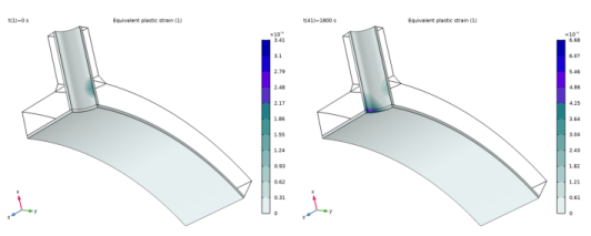
In the tree, select Study 3: Plasticity/Solution 3 (sol3) > Solid Mechanics > Equivalent Plastic Strain (solid).
|
|
4
|
Click the Add Result Template button in the window toolbar.
|
|
5
|
|
1
|
|
2
|
|
3
|
|
4
|
|
5
|
|
6
|
|
7
|
|
1
|
|
2
|
Go to the Result Templates window.
|
|
3
|
In the tree, select Study 3: Plasticity/Solution 3 (sol3) > Heat Transfer in Solids > Temperature (ht).
|
|
4
|
Click the Add Result Template button in the window toolbar.
|
|
5
|
|
1
|
|
2
|
|
3
|
|
4
|
|
1
|
|
2
|
|
3
|
|
4
|
|
1
|
|
2
|
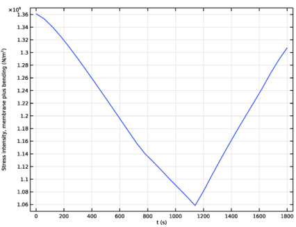
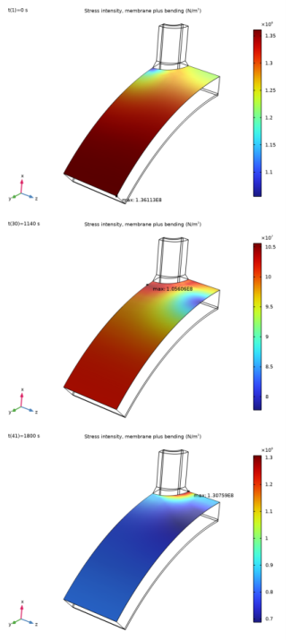
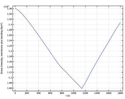
In the Settings window for Evaluation Group, type Stress Intensity, Maximum in the Label text field.
|
|
3
|
|
1
|
|
3
|
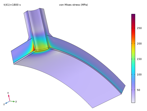
In the Settings window for Surface Maximum, click Replace Expression in the upper-right corner of the Expressions section. From the menu, choose Component 1 (comp1) > Solid Mechanics > Stress linearization > solid.SImb - Stress intensity, membrane plus bending - N/m².
|
|
4
|
|
5
|
|
1
|
Go to the Stress Intensity, Maximum window.
|
|
2
|
Click the Table Graph button in the window toolbar.
|
|
1
|
|
2
|
|
1
|
|
2
|
|
3
|
|
4
|
|
5
|
|
1
|
|
2
|
|
3
|
|
4
|
|
5
|
|
1
|
|
2
|
In the Settings window for Surface, click Replace Expression in the upper-right corner of the Expression section. From the menu, choose Component 1 (comp1) > Solid Mechanics > Stress linearization > solid.SImb - Stress intensity, membrane plus bending - N/m².
|
|
1
|
|
2
|
|
3
|
|
4
|
|
1
|
|
2
|
|
3
|
|
4
|
|
5
|
|
6
|
|
7
|
In the Graphics window, click on the maximum value marker. This automatically populates the Evaluation 3D table with the coordinates and the value of the plotted expression.
|
|
8
|
In the Evaluation 3D table, right-click on the newly added values and select Copy Selection to Clipboard.
|
|
1
|
In the Model Builder window, under Component 1 (comp1) > Solid Mechanics (solid) click Stress Linearization 1.
|
|
2
|
|
3
|
Select the Linearization line, starting point table and press CTRL+V. This inserts the coordinates into the table.
|
|
1
|
|
2
|
|
3
|
|
4
|
|
5
|
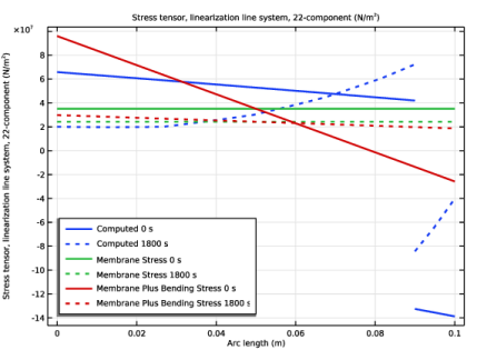
Locate the Legends section. Find the Include in automatic mode subsection. Clear the Point checkbox.
|
|
6
|
Select the Label checkbox.
|
|
1
|
|
2
|
|
3
|
|
4
|
|
5
|
Click to expand the Style Configuration section. From the Configuration list, choose Graph Plot Style 1.
|
|
6
|
|
7
|
|
1
|
|
2
|
In the Select Physics tree, select Structural Mechanics > Thermal–Structure Interaction > Thermal Stress, Solid.
|
|
3
|
Click Add.
|
|
4
|
Click
|
|
5
|
|
6
|
Click
|
|
1
|
|
2
|
|
3
|
|
4
|
|
5
|
Click
|
|
1
|
|
2
|
|
3
|
|
4
|
|
5
|
|
6
|
Click
|
|
1
|
|
2
|
|
3
|
|
4
|
|
5
|
|
6
|
|
7
|
|
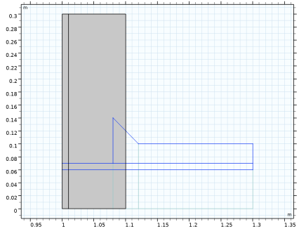
1
|
In the Model Builder window, under Component 1 (comp1) > Geometry 1 right-click Work Plane 1 (wp1) and choose Revolve.
|
|
2
|
|
3
|
|
4
|
|
5
|
|
6
|
|
7
|
Click
|
|
1
|
|
2
|
|
3
|
|
4
|
|
5
|
Click
|
|
1
|
|
2
|
|
3
|
|
4
|
|
5
|
|
6
|
Click
|
|
1
|
|
2
|
|
3
|
|
4
|
|
5
|
|
6
|
|
1
|
In the Model Builder window, under Component 1 (comp1) > Geometry 1 right-click Work Plane 2 (wp2) and choose Revolve.
|
|
2
|
|
3
|
Click the Angles button.
|
|
4
|
|
5
|
Click
|
|
6
|
|
1
|
|
2
|
|
3
|
Select the Keep objects to subtract checkbox.
|
|
4
|
Clear the Keep interior boundaries checkbox.
|
|
5
|
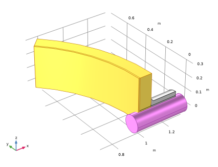
Select the object rev1(2) only.
|
|
6
|
|
7
|
|
8
|
Click
|
|
1
|
|
2
|
|
3
|
Select the Keep objects to subtract checkbox.
|
|
4
|
Select the object rev1(1) only.
|
|
5
|
|
6
|
|
7
|
Click
|
|
1
|
|
2
|
|
3
|
|
4
|
|
5
|
|
6
|
|
7
|
|
8
|
|
9
|
Click
|
|
1
|
|
2
|
|
3
|
|
4
|
|
5
|
|
6
|
Click
|
|
1
|
|
2
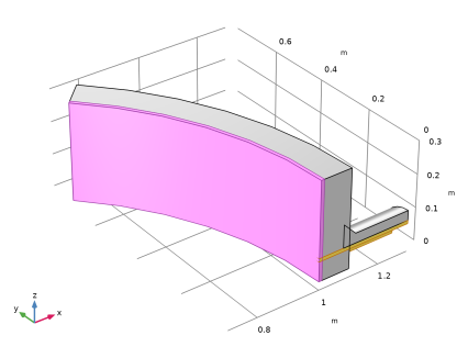
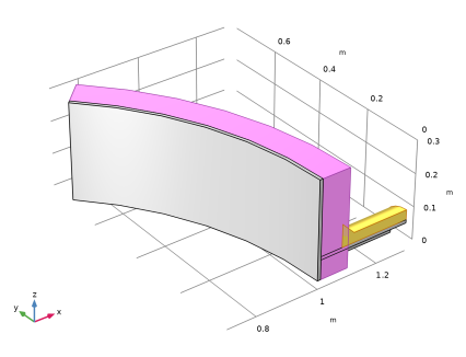
|
Select the object dif3 only.
|
|
3
|
|
4
|
|
5
|
Select the object dif1 only.
|
|
6
|
|
7
|
Click
|
|
8
|
|
9
|