COMSOL 6.4 - Tensile Test with Strain Rate Dependent Plasticity

Tensile Test with Strain Rate Dependent Plasticity

When a metal is deformed plastically at a high strain rate, the hardening function will exhibit higher values than at quasistatic conditions. That is, a higher stress is reached for a certain strain.

In this example, the Johnson–Cook material model is used to simulate this behavior for a tensile test run at different loading rates. The current yield stress σys is in this model described by Equation 1.

(1)

Here, σys0, k, n, C, and

are material parameters. The function f(Th) describes the temperature softening, where Th is a normalized temperature. It is often expressed as

where m is a material parameter.

The current yield stress is a product of three factors:

•

A standard strain hardening of the Ludvik form, with two parameters (k and n)

•

A strain rate dependent factor with two parameters (C and

). The reference strain rate

is the one at which k and n are determined

•

A temperature-dependent factor for softening. The reference temperature used to define Th is typically the one at which k and n are determined

Two different studies are performed to quantify the influence of the three factors. In the first study, both strain rate hardening and temperature softening are included, while in the second study, only the strain rate hardening is considered. In the model, four different values of the strain rate are investigated.

The analysis is coupled to a heat-transfer analysis, in which the heating caused by the plastic deformation is included. Due to this, the temperature will increase during the process, which is the source of the thermal softening.

Model Definition

Geometry

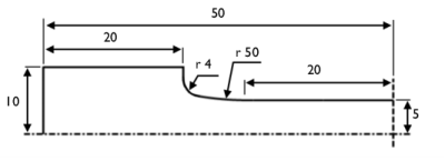
A 100 mm long cylindrical test specimen having a diameter of 10 mm in its central section is used. The detailed geometry is shown in Figure 1.

Figure 1: Geometry of the test specimen.

Axisymmetry is assumed, and only one half of the specimen is modeled due to the symmetry in the axial direction.

Material Model

The material is steel with properties as shown in Table 1.

Table 1: Material Properties.
Property	Symbol	Value
Young’s Modulus	E	200 GPa
Poisson’s ratio	ν	0.3
Coefficient of thermal expansion	α	12.3·10-61/K
Initial yield strength	σys0	400 MPa
Strength coefficient	k	200 MPa
Hardening exponent	n	0.5
Reference strain rate		1 1/s
Strain rate strength coefficient	C	0.12
Temperature exponent	m	0.6
Reference temperature	Tref	293.15 K
Melting temperature	Tm	1700 K
Thermal conductivity	k	44.5 W/(m·K)
Mass density	ρ	7850 kg/m3
Heat capacity at constant pressure	cp	475 J/(kg·K)

Boundary conditions

Mechanical

At the thick end of the specimen, the displacement is prescribed in the axial direction. The displacement varies linearly with time, and the maximum elongation of the specimen is 10 mm. This elongation corresponds to an average strain of 10%, but since the plastic deformation occurs only in the thinner part of the specimen, the actual plastic strains will be of the order 20%.

Symmetry conditions are applied in the axial direction at the symmetry plane.

Thermal

On all external boundaries, free convection to external room temperature (293.15 K) is assumed. The heat transfer coefficient is assumed to be 15 W/(m2·K).

Heat Generation

The inelastic deformation causes heat generation. The generated power per unit volume is the product of stress and the rate of plastic strain:

(2)

This power is used as a source term in the heat transfer analysis through the multiphysics coupling.

Thermal Expansion

Due to the heating, there will also be some thermal expansion of the specimen. This is included in the analysis through the multiphysics coupling, even though the effect is not large. The ratio between thermal and plastic strain can be used to quantify its influence. It can be estimated if the heat produced by plastic dissipation is assumed not to be conducted away from where it is generated:

(3)

Results and Discussion

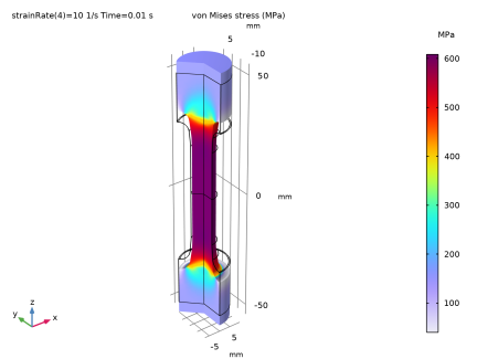
In Figure 2, a general overview of the stress state is shown for the highest loading rate in the first study. The stress in the central part is about 600 MPa, whereas the initial yield stress is 400 MPa. It can be found that the plastic strain at this stage is approximately 20%, and the contributions to the current stress can be estimated from Equation 1 as

(400 MPa + 200 MPa·0.20.5)(1+0.12·log(29))(1-0.0250.6) = 489 MPa · 1.36 · 0.89

Thus, there is about 22% strain hardening, 36% strain rate hardening, and 11% temperature softening.

Figure 2: Distribution of von Mises stress at the end of the tensile test at the highest strain rate.

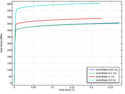
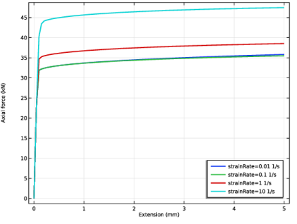
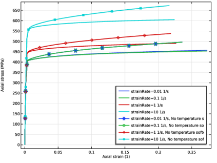
The influence of the strain rate is shown in Figure 3. The axial stress at the center of the bar is plotted as a function of the axial strain. Since the stress state is close to uniaxial, this graph essentially shows the constitutive law. For the two lower strain rates, the strain rate hardening effect is negligible since these are below the reference strain rate. It becomes significant when the average strain rate approaches 1/s. Figure 4 shows a corresponding graph of what would be measured in a testing machine, that is the total force versus the end point displacement.

Figure 3: Axial stress and strain at the center of the test specimen for the four tensile tests at different strain rates.

Figure 4: Force versus displacement for the four tensile tests at different strain rates.

In the second study, the temperature softening part of the constitutive law is switched off. The effect on the stress–strain relation is shown in Figure 5. Without the thermal softening effect, the hardening is much more pronounced. It can also be noted that the curves for the two lowest strain rates now completely coincide. The small difference that could be seen in Figure 3 was an effect of heating only.

Figure 5: Comparison of stress vs. strain with and without thermal softening.

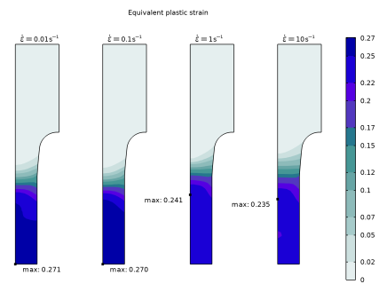
In Figure 6, the plastic strain distribution at the end of the experiment is shown for all four loading rates in the first study. At the lower strain rates, the maximum plastic deformation occurs in the central parts of the bar, whereas at the higher strain rates, the peak value actually occurs in a region closer to the loaded end. This redistribution is an effect of the thermal softening. The temperature will be higher at the center of the specimen at low loading rates.

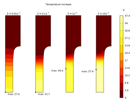
In Figure 7, the final temperature is shown. At the lowest loading rate, the whole process takes 100 s. There is thus enough time for a substantial redistribution of the temperature field. At the two highest loading rates, the temperature field to a large extent matches the strain distribution, since the time is not sufficient for any substantial diffusion of heat. The temperature is however higher at the highest loading rate, since the strain rate hardening causes a higher stress and thus a larger heat production for the same strain.

Figure 6: Distribution of plastic strain at the end of the process for all four strain rates.

Figure 7: Increase in temperature at the end of the process for all four strain rates.

Note that all analyses were performed using an assumption of geometric linearity in order to speed up the analysis and simplify comparisons. In reality, geometric nonlinearity should be taken into account; without it, the strain localization (“necking”) that may occur at the center of the bar cannot be predicted.

Nonlinear_Structural_Materials_Module/Plasticity/strain_rate_dependent_plasticity

Modeling Instructions

From the menu, choose .

New

In the window, click

Model Wizard

In the window, click

In the tree, select > > .

Click .

Click

In the tree, select > .

Click

Global Definitions

Parameters 1

In the window, under click .

In the window for , locate the section.

In the table, enter the following settings:


Name	Expression	Value	Description
totL	100[mm]	0.1 m	Total length of the specimen
avgStrain	0.1	0.1	Average strain
wMax	avgStrain*totL/2	0.005 m	Max displacement of the symmetric half
strainRate	0.1[1/s]	0.1 1/s	Strain rate
tFinal	avgStrain/strainRate	1 s	End time

Geometry 1

In the window, under click .

In the window for , locate the section.

From the list, choose .

Polygon 1 (pol1)

In the toolbar, click

In the window for , locate the section.

From the list, choose .

Locate the section. From the list, choose .

In the text field, type 5 5 0 0 10 10 6.01.

In the text field, type 20 0 0 50 50 30 30.

Quadratic Bézier 1 (qb1)

In the toolbar, click

and choose .

In the window for , locate the section.

In row , set to 6.01.

In row , set to 30.

In row , set to 5.25.

In row , set to 25.

In row , set to 5.

In row , set to 20.

Convert to Solid 1 (csol1)

In the toolbar, click

and choose .

Click in the window and then press Ctrl+A to select both objects.

In the window for , click

Fillet 1 (fil1)

In the toolbar, click

On the object , select Point 5 only.

In the window for , locate the section.

In the text field, type 4.

Click

Solid Mechanics (solid)

Symmetry Plane 1

In the toolbar, click

and choose .

Select Boundary 2 only.

Prescribed Displacement 1

In the toolbar, click

and choose .

Select Boundary 3 only.

In the window for , locate the section.

From the list, choose .

In the u 0 z text field, type wMax*t/tFinal.

Linear Elastic Material 1

In the window, click .

Plasticity 1

In the toolbar, click

and choose .

In the window for , locate the section.

Find the subsection. From the list, choose .

Materials

Structural steel

In the window, under right-click and choose .

In the window for , type Structural steel in the text field.

Locate the section. In the table, enter the following settings:


Property	Variable	Value	Unit	Property group
Young’s modulus	E	200[GPa]	Pa	Young’s modulus and Poisson’s ratio
Poisson’s ratio	nu	0.3	1	Young’s modulus and Poisson’s ratio
Density	rho	7850[kg/m^3]	kg/m³	Basic
Initial yield stress	sigmags	400[MPa]	Pa	Elastoplastic material model
Strength coefficient	k_jcook	200[MPa]	Pa	Johnson-Cook
Hardening exponent	n_jcook	0.5	1	Johnson-Cook
Reference strain rate	epet0_jcook	1	1/s	Johnson-Cook
Strain rate strength coefficient	C_jcook	0.12	1	Johnson-Cook
Temperature exponent	m_jcook	0.6		Johnson-Cook
Thermal conductivity	k_iso ; kii = k_iso, kij = 0	44.5[W/(m*K)]	W/(m·K)	Basic
Heat capacity at constant pressure	Cp	475[J/(kg*K)]	J/(kg·K)	Basic
Coefficient of thermal expansion	alpha_iso ; alphaii = alpha_iso, alphaij = 0	12.3e-6[1/K]	1/K	Basic