PDF

Small Punch Test for Ultrahigh Molecular Weight Polyethylene
Introduction
Ultrahigh Molecular Weight (UHMW) Polyethylene is a material commonly employed in knee and hip joint replacements. The “small punch test” is designed to assess mechanical properties using very small samples, which because of their reduced size can be directly explanted. This example demonstrates the use of the Bergstrom–Bischoff material model in the Polymer Viscoplasticity feature available in the Nonlinear Structural Materials Module.
Model Definition
In this model, a cylindrical test sample with a height, H, of 0.5 mm and a diameter, D, of 6.4 mm, is subjected to a biaxial state of tension by a hemispherical punch moving at a constant speed of 0.5 mm/min. Both the loading and unloading phases are modeled in the numerical simulation.
The geometry exhibits 2D axial symmetry. It is therefore possible to reduce the model geometry of the specimen to a rectangle with a width equal to its radius.
Material Model
The rheology of the Bergstrom–Bischoff material model is shown in Figure 1. It features a so-called equilibrium network that can be schematized as a hyperelastic spring characterized by an Arruda–Boyce strain energy, augmented with a first order dependence on the second invariant of the isochoric elastic Cauchy–Green deformation tensor as in Ref. 1. The Cauchy stress is thus computed as
(1)
where σAB is the stress computed from a standard Arruda–Boyce hyperelastic material with quadratic, uncoupled volumetric strain energy, q is a weight on the relative contribution of the second isochoric invariant, J is the determinant of the deformation gradient, b is the isochoric left Cauchy–Green tensor, and I the second-order identity tensor. The material property μi is the initial shear modulus, which is related to the macroscopic shear modulus μ appearing in the five-terms Arruda–Boyce hyperelastic strain energy as (Ref. 2)
where N is the number of segments and L1 is the inverse Langevin function. Two more networks in parallel with the equilibrium network model the nonequilibrium behavior. Each of the latter networks comprises an isochoric standard Arruda–Boyce spring in series with a viscoplastic element whose rate multiplier is given by
(2)
where σvm is the von Mises stress of the nonequilibrium network and A, ai, ni, and σres,i identify material properties. The shear modulus of the nonequilibrium networks is set by an energy factor βvi that represents the relative stiffness of the each nonequilibrium network with respect to the equilibrium one. The energy factor of the second nonequilibrium network is made dependent on the viscoplastic strain of the first one by the differential equation
where α and βv,f are material properties.
The numerical values of the material properties used in the model are adapted from those used in Ref. 1 for the COMSOL Multiphysics implementation of the Bergstrom–Bischoff model.
Figure 1: Rheology of the Bergstrom–Bischoff material model.
Results and Discussion
Figure 2 shows the force versus punch displacement curve. The model is able to reproduce the failure of the specimen that occurs at a punch displacement of approximately 2.4 mm. The punch force drops to zero during the unloading phase when it detaches from the specimen as a consequence of the viscoplastic deformation accumulated during the test.
Figure 3 shows the deformed shape of the specimen at the end of the simulation. The color highlights the first principal strain, where a circular region characterized by biaxial necking can be observed.
Figure 2: Force versus punch displacement curve.
Figure 3: First principal strain in the specimen after the unloading phase.
Notes About the COMSOL Implementation
The punch and the clamp are modeled as rigid bodies. The punch goes forward and backward at constant speed. The corresponding displacement can be imposed by defining a Triangle function found under Definitions. To facilitate convergence of the nonlinear solver, the Smoothing option is used, such that the resulting time history has at least two continuous derivatives. This is important not only at the time instant when the speed changes sign, but also at the initial time, in order to gradually start from zero speed. This allows to impose a motion that is consistent with the initial condition prescribing zero velocity.
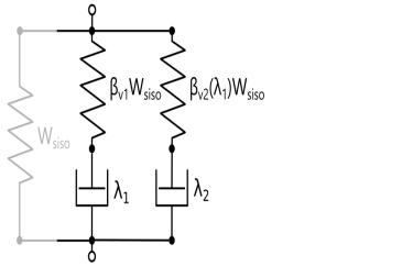
The External stress feature under Hyperelastic Material allows you to include the extra terms in the stress definition of the equilibrium network:
Note that while the second term can be easily added as an isotropic Cauchy stress, the first and the third terms are most easily added by computing the corresponding Second Piola–Kirchhoff stress tensor. Indeed, the first term becomes isotropic
(3)
and the third can be expressed using the right Cauchy-Green deformation tensor C
You can use the Bergstrom–Bischoff material model by adding a Polymer Viscoplasticity node under Hyperelastic Material.
You find the Domain ODEs option in the Time stepping section of the Polymer Viscoplasticity node. This option can be faster than Backward Euler when the size of the problem is small.
References
1. J.S. Bergström and J.E. Bischoff, “An Advanced Thermomechanical Constitutive Model for UHMWPE,” International Journal of Structural Changes in Solids, vol. 2, no. 1, pp. 31–39, 2010.
2. J.S. Bergström, Mechanics of Solid polymers: Theory and Computational Modeling, William Andrew, 2015.
3. J.S. Bergström and N. Elabbasi, “Nonlinear Mechanical Modeling of Thermoplastics,” COMSOL Conference, 2016.
Application Library path: Nonlinear_Structural_Materials_Module/Viscoplasticity/small_punch_test
Modeling Instructions
From the File menu, choose New.
New
In the New window, click  Model Wizard.
Model Wizard
1
In the Model Wizard window, click  2D Axisymmetric.
2
In the Select Physics tree, select Structural Mechanics > Solid Mechanics (solid).
3
Click Add.
4
Click  Study.
5
In the Select Study tree, select General Studies > Time Dependent.
6
Global Definitions
Geometrical Parameters
1
In the Model Builder window, under Global Definitions click Parameters 1.
2
In the Settings window for Parameters, locate the Parameters section.
3
Click  Load from File.
4
5
In the Label text field, type Geometrical Parameters.
Geometry 1
The geometry sequence for the model is available in a file. If you want to create it from scratch yourself, you can follow the instructions in the Appendix — Geometry Modeling Instructions section. Otherwise, insert the geometry sequence as follows:
1
In the Geometry toolbar, click Insert Sequence and choose Insert Sequence.
2
3
In the Geometry toolbar, click  Build All.
Now set up the contact pairs. Choose as source of the pair the boundaries on the domains that will be modeled as rigid.
Definitions
Contact Pair 1 (ap1)
1
In the Model Builder window, expand the Definitions node, then click Contact Pair 1 (ap1).
2
In the Settings window for Pair, click the  Swap Source and Destination button.
Contact Pair 2 (ap2)
1
In the Model Builder window, click Contact Pair 2 (ap2).
2
In the Settings window for Pair, click the  Swap Source and Destination button.
3
Locate the Source Boundaries section. Click to select the  Activate Selection toggle button.
4
Locate the Pair Type section. Select the Manual control of selections and pair type checkbox.
5
6
Click the  Zoom Extents button in the Graphics toolbar.
Contact Pair 3 (p3)
1
In the Definitions toolbar, click  Pairs and choose Contact Pair.
2
3
In the Settings window for Pair, locate the Destination Boundaries section.
4
Click to select the  Activate Selection toggle button.
5
Set up the material models.
Global Definitions
Material Parameters
1
In the Home toolbar, click  Parameters and choose Add > Parameters.
2
In the Settings window for Parameters, locate the Parameters section.
3
Click  Load from File.
4
5
In the Label text field, type Material Parameters.
Solid Mechanics (solid)
Hyperelastic Material 1
1
In the Physics toolbar, click  Domains and choose Hyperelastic Material.
2
3
In the Settings window for Hyperelastic Material, locate the Hyperelastic Material section.
4
From the Material model list, choose Arruda–Boyce.
5
From the Compressibility list, choose Compressible, uncoupled.
6
Locate the Quadrature Settings section. Select the Reduced integration checkbox.
7
Click the  Show More Options button in the Model Builder toolbar.
8
In the Show More Options dialog, in the tree, select the checkbox for the node Physics > Advanced Physics Options.
9
10
In the Settings window for Hyperelastic Material, click to expand the Energy Dissipation section.
11
From the Store dissipation list, choose Domain ODEs (legacy).
Polymer Viscoplasticity 1
1
In the Physics toolbar, click  Attributes and choose Polymer Viscoplasticity.
2
In the Settings window for Polymer Viscoplasticity, locate the Viscoplasticity Model section.
3
From the Material model list, choose Bergstrom–Bischoff.
4
Find the Network 1 subsection. In the βv1 text field, type betav1/(1/(1+q)).
5
Find the Network 2 subsection. In the βv,  i text field, type betav2_i/(1/(1+q)).
6
In the βv,  f text field, type betav2_f/(1/(1+q)).
7
In the α text field, type alfa_rate.
8
Locate the Time Stepping section. From the Method list, choose Domain ODEs.
Materials
UHMWPE
1
In the Model Builder window, under Component 1 (comp1) right-click Materials and choose Blank Material.
2
3
In the Settings window for Material, type UHMWPE in the Label text field.
4
Locate the Material Contents section. In the table, enter the following settings:
The stress exponents of the Bergstrom–Bischoff model is reduced for small times to help initialize the solution.
Solid Mechanics (solid)
Hyperelastic Material 1
In the Model Builder window, under Component 1 (comp1) > Solid Mechanics (solid) click Hyperelastic Material 1.
External Stress 1
1
In the Physics toolbar, click  Attributes and choose External Stress.
2
In the Settings window for External Stress, locate the External Stress section.
3
In the Sext text field, type q/(1+q)*mu_initial*solid.J^(-2/3)*solid.I1CIel.
Hyperelastic Material 1
In the Model Builder window, click Hyperelastic Material 1.
External Stress 2
1
In the Physics toolbar, click  Attributes and choose External Stress.
2
In the Settings window for External Stress, locate the External Stress section.
3
From the Stress input list, choose Stress tensor (Spatial).
4
In the σext text field, type -(2/3)*q/(1+q)*mu_initial*solid.I2CIel/solid.J.
Hyperelastic Material 1
In the Model Builder window, click Hyperelastic Material 1.
External Stress 3
1
In the Physics toolbar, click  Attributes and choose External Stress.
2
In the Settings window for External Stress, locate the External Stress section.
3
4
Specify the Sext matrix as
Materials
Steel
1
In the Model Builder window, under Component 1 (comp1) right-click Materials and choose Blank Material.
2
3
In the Settings window for Material, type Steel in the Label text field.
4
Locate the Material Contents section. In the table, enter the following settings:
Solid Mechanics (solid)
Rigid Material: Clamp
1
In the Physics toolbar, click  Domains and choose Rigid Material.
2
In the Settings window for Rigid Material, type Rigid Material: Clamp in the Label text field.
3
Fixed Constraint 1
In the Physics toolbar, click  Attributes and choose Fixed Constraint.
Rigid Material: Punch
1
In the Physics toolbar, click  Domains and choose Rigid Material.
2
3
In the Settings window for Rigid Material, type Rigid Material: Punch in the Label text field.
Define the imposed displacement for the punch.
Global Definitions
Test Parameters
1
In the Home toolbar, click  Parameters and choose Add > Parameters.
2
In the Settings window for Parameters, type Test Parameters in the Label text field.
3
Locate the Parameters section. In the table, enter the following settings:
Definitions
Punch Displacement
1
In the Definitions toolbar, click  More Functions and choose Triangle.
2
In the Settings window for Triangle, type Punch Displacement in the Label text field.
3
Locate the Parameters section. In the Lower limit text field, type Dt_transient.
4
In the Upper limit text field, type Dt_tot.
5
In the Amplitude text field, type wmax.
6
Click to expand the Smoothing section. In the Size of transition zone text field, type 20[s].
7
Solid Mechanics (solid)
Rigid Material: Punch
In the Model Builder window, under Component 1 (comp1) > Solid Mechanics (solid) click Rigid Material: Punch.
Prescribed Displacement/Rotation 1
1
In the Physics toolbar, click  Attributes and choose Prescribed Displacement/Rotation.
2
In the Settings window for Prescribed Displacement/Rotation, locate the Prescribed Displacement section.
3
In the w0 text field, type tri1(t).
Enable Evaluate of reaction forces to compute the punch reaction force.
4
Click to expand the Reaction Force Settings section. Select the Evaluate reaction forces using weak constraints checkbox.
Inertia forces are negligible.
5
In the Model Builder window, click Solid Mechanics (solid).
6
In the Settings window for Solid Mechanics, locate the Structural Transient Behavior section.
7
Adjust the contact settings.
Contact 1
1
In the Model Builder window, under Component 1 (comp1) > Solid Mechanics (solid) click Contact 1.
2
In the Settings window for Contact, click to expand the Advanced section.
3
In the Echar text field, type solid.Eequ*(1+betav1+betav2_i).
Friction 1
1
In the Physics toolbar, click  Attributes and choose Friction.
2
In the Settings window for Friction, locate the Friction Parameters section.
3
In the μ text field, type 0.05.
4
Locate the Friction Force Penalty Factor section. From the Penalty factor control list, choose Manual tuning.
5
In the ft text field, type 0.1.
Set up the mesh.
Global Definitions
Mesh Parameters
1
In the Home toolbar, click  Parameters and choose Add > Parameters.
2
In the Settings window for Parameters, type Mesh Parameters in the Label text field.
3
Locate the Parameters section. In the table, enter the following settings:
Draw partitions in order to improve the mesh.
Geometry 1
Rectangle 5 (r5)
1
In the Geometry toolbar, click  Rectangle.
2
In the Settings window for Rectangle, locate the Size and Shape section.
3
In the Width text field, type w_mesh*8.
4
In the Height text field, type th_mesh*2.
5
Locate the Position section. In the r text field, type w_mesh*28.
6
In the z text field, type th-th_mesh*2.
7
Click  Build Selected.
Partition Domains 1 (pard1)
1
In the Geometry toolbar, click  Booleans and Partitions and choose Partition Domains.
2
On the object r1, select Domain 1 only.
3
In the Settings window for Partition Domains, locate the Partition Domains section.
4
From the Partition with list, choose Objects.
5
6
Clear the Keep objects checkbox.
7
Click  Build Selected.
Rectangle 6 (r6)
1
In the Geometry toolbar, click  Rectangle.
2
In the Settings window for Rectangle, locate the Size and Shape section.
3
In the Width text field, type D/2.
4
In the Height text field, type th_mesh*2.
5
Locate the Position section. In the z text field, type th-th_mesh*2.
6
Click  Build Selected.
Partition Domains 2 (pard2)
1
In the Model Builder window, under Component 1 (comp1) > Geometry 1 right-click Partition Domains 1 (pard1) and choose Duplicate.
2
In the Settings window for Partition Domains, locate the Partition Domains section.
3
Click to select the  Activate Selection toggle button for Domains to partition.
4
On the object pard1, select Domain 1 only.
5
Click to select the  Activate Selection toggle button for Objects.
6
7
Click  Build Selected.
Mesh Control Edges 1 (mce1)
1
In the Model Builder window, click Mesh Control Edges 1 (mce1).
2
In the Settings window for Mesh Control Edges, locate the Input section.
3
Click to select the  Activate Selection toggle button for Edges to include.
4
On the object fin, select Boundaries 4, 10, 12, 13, 15, and 16 only.
Mesh 1
Mapped 1
1
In the Mesh toolbar, click  Mapped.
2
In the Settings window for Mapped, locate the Domain Selection section.
3
From the Geometric entity level list, choose Domain.
4
Distribution 1
1
Right-click Mapped 1 and choose Distribution.
2
3
In the Settings window for Distribution, locate the Distribution section.
4
In the Number of elements text field, type 8.
Distribution 2
1
In the Model Builder window, right-click Mapped 1 and choose Distribution.
2
3
In the Settings window for Distribution, locate the Distribution section.
4
In the Number of elements text field, type 2.
5
Click  Build Selected.
Convert 1
1
In the Mesh toolbar, click  Modify and choose Convert.
2
In the Settings window for Convert, locate the Element Split Method section.
3
From the Element split method list, choose Insert centerpoints.
4
Locate the Domain Selection section. From the Geometric entity level list, choose Domain.
5
6
Click  Build Selected.
Mapped 2
1
In the Mesh toolbar, click  Mapped.
2
In the Settings window for Mapped, locate the Domain Selection section.
3
From the Geometric entity level list, choose Domain.
4
5
Click to expand the Control Entities section. From the Smooth across removed control entities list, choose Off.
Distribution 1
1
Right-click Mapped 2 and choose Distribution.
2
3
In the Settings window for Distribution, locate the Distribution section.
4
In the Number of elements text field, type 50.
Distribution 2
1
In the Model Builder window, right-click Mapped 2 and choose Distribution.
2
3
In the Settings window for Distribution, locate the Distribution section.
4
In the Number of elements text field, type 6.
Distribution 3
1
Right-click Mapped 2 and choose Distribution.
2
3
In the Settings window for Distribution, locate the Distribution section.
4
In the Number of elements text field, type 2.
5
Click  Build Selected.
Mapped 3
1
In the Mesh toolbar, click  Mapped.
2
In the Settings window for Mapped, locate the Domain Selection section.
3
From the Geometric entity level list, choose Domain.
4
Distribution 1
1
Right-click Mapped 3 and choose Distribution.
2
3
In the Settings window for Distribution, locate the Distribution section.
4
In the Number of elements text field, type 1.
5
Click  Build Selected.
Free Triangular 1
1
In the Mesh toolbar, click  Free Triangular.
2
In the Settings window for Free Triangular, click to expand the Control Entities section.
3
From the Smooth across removed control entities list, choose Off.
Size
1
In the Model Builder window, click Size.
2
In the Settings window for Size, locate the Element Size section.
3
From the Predefined list, choose Finer.
4
Click  Build All.
Study 1
1
In the Model Builder window, click Study 1.
2
In the Settings window for Study, locate the Study Settings section.
3
Clear the Generate default plots checkbox.
Step 1: Time Dependent
1
In the Model Builder window, under Study 1 click Step 1: Time Dependent.
2
In the Settings window for Time Dependent, locate the Study Settings section.
3
In the Output times text field, type range(0,2,Dt_tot).
Solution 1 (sol1)
1
In the Study toolbar, click  Show Default Solver.
2
In the Model Builder window, expand the Solution 1 (sol1) node.
3
In the Model Builder window, expand the Study 1 > Solver Configurations > Solution 1 (sol1) > Dependent Variables 1 node, then click Viscoplastic Strain Tensor, Local Coordinate System (comp1.solid.hmm1.pvp1.evp1).
4
In the Settings window for Field, locate the Scaling section.
5
From the Method list, choose Manual.
6
In the Scale text field, type 3.
7
In the Model Builder window, under Study 1 > Solver Configurations > Solution 1 (sol1) > Dependent Variables 1 click Viscoplastic Strain Tensor, Local Coordinate System (comp1.solid.hmm1.pvp1.evp2).
8
In the Settings window for Field, locate the Scaling section.
9
From the Method list, choose Manual.
10
In the Scale text field, type 3.
11
In the Model Builder window, under Study 1 > Solver Configurations > Solution 1 (sol1) > Dependent Variables 1 click Equivalent Viscoplastic Strain, Network 1 (comp1.solid.hmm1.pvp1.evpe1).
12
In the Settings window for Field, locate the Scaling section.
13
From the Method list, choose Manual.
14
In the Scale text field, type 3.
15
In the Model Builder window, under Study 1 > Solver Configurations > Solution 1 (sol1) > Dependent Variables 1 click Equivalent Viscoplastic Strain, Network 2 (comp1.solid.hmm1.pvp1.evpe2).
16
In the Settings window for Field, locate the Scaling section.
17
From the Method list, choose Manual.
18
In the Scale text field, type 3.
19
In the Model Builder window, under Study 1 > Solver Configurations > Solution 1 (sol1) > Dependent Variables 1 click Displacement Field (comp1.u).
20
In the Settings window for Field, locate the Scaling section.
21
In the Scale text field, type 4[mm].
22
In the Model Builder window, under Study 1 > Solver Configurations > Solution 1 (sol1) > Dependent Variables 1 click Rigid Material Displacements (comp1.solid_rd_disp).
23
In the Settings window for State, locate the Scaling section.
24
In the Scale text field, type 4[mm].
25
In the Model Builder window, under Study 1 > Solver Configurations > Solution 1 (sol1) > Dependent Variables 1 click Reaction Force (comp1.solid.rd2.RFz).
26
In the Settings window for State, locate the Scaling section.
27
From the Method list, choose Manual.
28
In the Scale text field, type 100.
29
In the Model Builder window, under Study 1 > Solver Configurations > Solution 1 (sol1) > Dependent Variables 1 click Viscoplastic Dissipation Density (comp1.solid.Wvp).
30
In the Settings window for Field, locate the Scaling section.
31
From the Method list, choose Manual.
32
In the Scale text field, type 1.0E7.
33
In the Model Builder window, under Study 1 > Solver Configurations > Solution 1 (sol1) click Time-Dependent Solver 1.
34
In the Settings window for Time-Dependent Solver, click to expand the Time Stepping section.
35
From the Steps taken by solver list, choose Strict.
36
In the Model Builder window, expand the Study 1 > Solver Configurations > Solution 1 (sol1) > Time-Dependent Solver 1 node, then click Direct.
37
In the Settings window for Direct, locate the General section.
38
From the Solver list, choose PARDISO.
39
In the Model Builder window, under Study 1 > Solver Configurations > Solution 1 (sol1) > Time-Dependent Solver 1 click Fully Coupled 1.
40
In the Settings window for Fully Coupled, click to expand the Method and Termination section.
41
In the Minimum damping factor text field, type 0.3.
42
In the Maximum number of iterations text field, type 20.
43
In the Study toolbar, click  Get Initial Value.
Results
In the Model Builder window, expand the Results node.
Displacement Magnitude
1
In the Model Builder window, expand the Results > Datasets node.
2
Right-click Results and choose 2D Plot Group.
3
In the Settings window for 2D Plot Group, type Displacement Magnitude in the Label text field.
4
Locate the Plot Settings section. From the Frame list, choose Spatial  (r, phi, z).
Polymer
1
Right-click Displacement Magnitude and choose Surface.
2
In the Settings window for Surface, type Polymer in the Label text field.
Selection 1
1
Right-click Polymer and choose Selection.
2
Deformation 1
1
In the Model Builder window, right-click Polymer and choose Deformation.
2
In the Settings window for Deformation, locate the Scale section.
3
Select the Scale factor checkbox. In the associated text field, type 1.
Punch and Clamp
1
In the Model Builder window, right-click Displacement Magnitude and choose Surface.
2
In the Settings window for Surface, type Punch and Clamp in the Label text field.
3
Click to expand the Title section. From the Title type list, choose None.
4
Locate the Expression section. In the Expression text field, type 1.
5
Locate the Coloring and Style section. From the Coloring list, choose Uniform.
6
From the Color list, choose Gray.
Selection 1
1
Right-click Punch and Clamp and choose Selection.
2
Deformation 1
1
In the Model Builder window, right-click Punch and Clamp and choose Deformation.
2
In the Settings window for Deformation, locate the Scale section.
3
Select the Scale factor checkbox. In the associated text field, type 1.
Study 1
Step 1: Time Dependent
1
In the Model Builder window, under Study 1 click Step 1: Time Dependent.
2
In the Settings window for Time Dependent, click to expand the Results While Solving section.
3
Select the Plot checkbox.
4
In the Study toolbar, click  Compute.
5
Click the  Zoom Extents button in the Graphics toolbar.
Results
Punch Force
1
In the Results toolbar, click  1D Plot Group.
2
In the Settings window for 1D Plot Group, type Punch Force in the Label text field.
3
Click to expand the Title section. From the Title type list, choose Manual.
4
In the Title text area, type Punch Contact Force.
5
Locate the Plot Settings section.
6
Select the x-axis label checkbox. In the associated text field, type Punch displacement (mm).
7
Select the y-axis label checkbox. In the associated text field, type Punch force (N).
8
Locate the Grid section. Select the Manual spacing checkbox.
9
In the x spacing text field, type 0.5.
10
In the y spacing text field, type 20.
11
Locate the Legend section. From the Position list, choose Upper left.
Global 1
1
Right-click Punch Force and choose Global.
2
In the Settings window for Global, locate the y-Axis Data section.
3
4
Locate the x-Axis Data section. From the Parameter list, choose Expression.
5
In the Expression text field, type tri1(t).
6
Click to expand the Coloring and Style section. From the Width list, choose 2.
Import numerical data from Ref. 1 for comparison.
Reference
1
In the Results toolbar, click  Table.
2
In the Settings window for Table, type Reference in the Label text field.
3
Locate the Data section. Click  Import.
4
Reference
1
In the Model Builder window, right-click Punch Force and choose Table Graph.
2
In the Settings window for Table Graph, type Reference in the Label text field.
3
Locate the Coloring and Style section. Find the Line style subsection. From the Line list, choose None.
4
Find the Line markers subsection. From the Marker list, choose Circle.
5
Click to expand the Legends section. Select the Show legends checkbox.
6
Find the Include subsection. Select the Label checkbox.
7
Clear the Headers checkbox.
COMSOL
1
In the Model Builder window, under Results > Punch Force click Global 1.
2
In the Settings window for Global, type COMSOL in the Label text field.
3
Click to expand the Legends section. Find the Include subsection. Select the Label checkbox.
4
Clear the Solution checkbox.
5
Clear the Description checkbox.
6
In the Punch Force toolbar, click  Plot.
Dissipated Energy
1
In the Results toolbar, click  1D Plot Group.
2
In the Settings window for 1D Plot Group, type Dissipated Energy in the Label text field.
3
Locate the Title section. From the Title type list, choose Manual.
4
In the Title text area, type Dissipated Energy.
Global 1
1
Right-click Dissipated Energy and choose Global.
2
In the Settings window for Global, click Replace Expression in the upper-right corner of the y-Axis Data section. From the menu, choose Component 1 (comp1) > Solid Mechanics > Global > solid.Wvp_tot - Total viscoplastic dissipation - J.
3
Locate the x-Axis Data section. From the Parameter list, choose Expression.
4
In the Expression text field, type tri1(t).
5
Locate the Coloring and Style section. From the Width list, choose 2.
6
Locate the Legends section. Clear the Show legends checkbox.
7
In the Dissipated Energy toolbar, click  Plot.
Revolution 2D: Polymer
1
In the Results toolbar, click  More Datasets and choose Revolution 2D.
2
In the Settings window for Revolution 2D, type Revolution 2D: Polymer in the Label text field.
3
Click to expand the Revolution Layers section. In the Start angle text field, type -60.
4
In the Revolution angle text field, type 270.
Selection
1
In the Results toolbar, click  Attributes and choose Selection.
2
In the Settings window for Selection, locate the Geometric Entity Selection section.
3
From the Geometric entity level list, choose Domain.
4
First Principal Strain
1
In the Results toolbar, click  3D Plot Group.
2
In the Settings window for 3D Plot Group, type First Principal Strain in the Label text field.
3
Locate the Plot Settings section. Clear the Plot dataset edges checkbox.
4
Click to expand the Title section. From the Title type list, choose Label.
Polymer
1
Right-click First Principal Strain and choose Volume.
2
In the Settings window for Volume, locate the Expression section.
3
In the Expression text field, type solid.ep1.
4
Locate the Coloring and Style section. From the Color table list, choose Prism.
5
In the Label text field, type Polymer.
Deformation 1
1
Right-click Polymer and choose Deformation.
2
In the Settings window for Deformation, locate the Scale section.
3
Select the Scale factor checkbox. In the associated text field, type 1.
Revolution 2D: Punch
1
In the Model Builder window, right-click Revolution 2D: Polymer and choose Duplicate.
2
In the Settings window for Revolution 2D, type Revolution 2D: Punch in the Label text field.
3
Locate the Revolution Layers section. In the Start angle text field, type 0.
4
In the Revolution angle text field, type 360.
Selection
1
In the Model Builder window, expand the Revolution 2D: Punch node, then click Selection.
2
Punch
1
In the Model Builder window, right-click First Principal Strain and choose Surface.
2
In the Settings window for Surface, type Punch in the Label text field.
3
Locate the Data section. From the Dataset list, choose Revolution 2D: Punch.
4
From the Solution parameters list, choose From parent.
5
Locate the Expression section. In the Expression text field, type 1.
6
Locate the Coloring and Style section. From the Coloring list, choose Uniform.
7
From the Color list, choose Gray.
Deformation 1
1
Right-click Punch and choose Deformation.
2
In the Settings window for Deformation, locate the Scale section.
3
Select the Scale factor checkbox. In the associated text field, type 1.
Revolution 2D: Clamp
1
In the Model Builder window, right-click Revolution 2D: Punch and choose Duplicate.
2
In the Settings window for Revolution 2D, type Revolution 2D: Clamp in the Label text field.
3
Locate the Revolution Layers section. In the Start angle text field, type -60.
4
In the Revolution angle text field, type 270.
Selection
1
In the Model Builder window, expand the Revolution 2D: Clamp node, then click Selection.
2
Clamp
1
In the Model Builder window, right-click First Principal Strain and choose Volume.
2
In the Settings window for Volume, type Clamp in the Label text field.
3
Locate the Data section. From the Dataset list, choose Revolution 2D: Clamp.
4
From the Solution parameters list, choose From parent.
5
Locate the Expression section. In the Expression text field, type 1.
6
Locate the Coloring and Style section. From the Coloring list, choose Uniform.
7
From the Color list, choose Gray.
Material Appearance 1
1
Right-click Clamp and choose Material Appearance.
2
In the Settings window for Material Appearance, locate the Appearance section.
3
From the Appearance list, choose Custom.
4
From the Material type list, choose Steel (scratched).
5
In the First Principal Strain toolbar, click  Plot.
Appendix — Geometry Modeling Instructions
From the File menu, choose New.
New
In the New window, click  Model Wizard.
Model Wizard
1
In the Model Wizard window, click  2D Axisymmetric.
2
Global Definitions
Geometrical Parameters
1
In the Model Builder window, under Global Definitions click Parameters 1.
2
In the Settings window for Parameters, locate the Parameters section.
3
Click  Load from File.
4
5
In the Label text field, type Geometrical Parameters.
Geometry 1
1
In the Model Builder window, under Component 1 (comp1) click Geometry 1.
2
In the Settings window for Geometry, locate the Units section.
3
From the Length unit list, choose mm.
Rectangle 1 (r1)
1
In the Geometry toolbar, click  Rectangle.
2
In the Settings window for Rectangle, locate the Size and Shape section.
3
In the Width text field, type D/2.
4
In the Height text field, type th.
Rectangle 2 (r2)
1
In the Geometry toolbar, click  Rectangle.
2
In the Settings window for Rectangle, locate the Size and Shape section.
3
In the Width text field, type rout_clamp-r_bottom.
4
In the Height text field, type th/4.
5
Locate the Position section. In the r text field, type r_bottom.
6
In the z text field, type -th/4.
Rectangle 3 (r3)
1
In the Geometry toolbar, click  Rectangle.
2
In the Settings window for Rectangle, locate the Size and Shape section.
3
In the Width text field, type rout_clamp-r_top.
4
In the Height text field, type th.
5
Locate the Position section. In the r text field, type r_top.
6
In the z text field, type th.
Circle 1 (c1)
1
In the Geometry toolbar, click  Circle.
2
In the Settings window for Circle, locate the Size and Shape section.
3
In the Radius text field, type r_punch.
4
In the Sector angle text field, type 90.
5
Locate the Position section. In the z text field, type -r_punch.
Rectangle 4 (r4)
1
In the Geometry toolbar, click  Rectangle.
2
In the Settings window for Rectangle, locate the Size and Shape section.
3
In the Width text field, type r_punch.
4
In the Height text field, type h_punch-r_punch.
5
Locate the Position section. In the z text field, type -h_punch.
6
Click  Build Selected.
7
Click the  Zoom Extents button in the Graphics toolbar.
Fillet 1 (fil1)
1
In the Geometry toolbar, click  Fillet.
2
On the object r3, select Point 1 only.
3
In the Settings window for Fillet, locate the Radius section.
4
In the Radius text field, type r_fillet.
Union 1 (uni1)
1
In the Geometry toolbar, click  Booleans and Partitions and choose Union.
2
Select the objects c1 and r4 only.
3
In the Settings window for Union, click  Build Selected.
4
Click  Build Selected.
Form Union (fin)
1
In the Model Builder window, under Component 1 (comp1) > Geometry 1 click Form Union (fin).
2
In the Settings window for Form Union/Assembly, locate the Form Union/Assembly section.
3
From the Action list, choose Form an assembly.
4
From the Pair type list, choose Contact pair.
5
In the Geometry toolbar, click  Build All.
Mesh Control Edges 1 (mce1)
1
In the Geometry toolbar, click  Virtual Operations and choose Mesh Control Edges.
2
On the object fin, select Boundary 4 only.
3
In the Geometry toolbar, click  Build All.