PDF

Uniaxial Stretching of a Rectangular Sheet
Introduction
Wrinkling is a commonly occurring phenomenon in thin sheets, caused by either loading or manufacturing defects. The numerical treatment of wrinkles in thin structures can be approached using the following two theories:
Membrane theory along with tension field theory — Membrane theory models wrinkles as a mean surface and gives a correct stress distribution in the wrinkled region. This is computationally inexpensive compared to shell theory, but the wrinkle amplitudes and wavelengths cannot be obtained. An example of modeling wrinkling in a rectangular sheet using the Membrane interface can be found in the Structural Mechanics Module Application Library model Uniaxial Stretching of a Rectangular Membrane.
Shell theory — As wrinkling is a local buckling phenomenon, nonlinear postbuckling analysis is needed to find the amplitudes and wavelengths of the wrinkles. This modeling approach is nontrivial and computationally expensive.
In this example, wrinkling in a thin rectangular sheet is modeled using a shell theory. First, a static analysis is performed to determine the region of negative principal stresses without assuming wrinkles. The negative principal stress is a prerequisite for the occurrence of wrinkles. Next, a prestressed buckling analysis is carried out to find out the potential linearized buckling modes. Finally, a nonlinear postbuckling analysis is carried out to investigate the evolution of wrinkles. The example is taken from Ref. 1, with which the results obtained here are compared.
Model Definition
A rectangular sheet 25 cm in length, 10 cm in width, and 0.1 mm thick is stretched in the longitudinal direction.
One of the short edges is fixed, while a prescribed displacement is applied on the opposite edge. The long edges are unconstrained.
The sheet is made of an incompressible neo-Hookean hyperelastic material with a Lame parameter of 6 MPa.
Results and Discussions
The example is based on Ref. 1 and Ref. 2 with some modifications. The authors (see Ref. 2) used 100,000 quadrilateral mesh elements, whereas we use 12,500 elements to save computation time. The nominal strain at which wrinkling starts in the postbuckling analysis depends on the mesh distribution, as reported in Ref. 2 (although the variation is small). Also the buckling modes and the critical factor depend on the mesh distribution. The authors in Ref. 1 reported that the numerical results of the postbuckling analysis depends on the number of modes used as geometric imperfection, as well as on their amplitudes. They have considered four buckling modes and an amplitude equal to 0.1% of the sheet thickness. In this example, four buckling modes are also used but the amplitude varies for each mode. A lower factor is assigned to the higher modes to reduce their influence.
Figure 1 shows the regions of negative transverse stress, called wrinkled regions, for different values of the nominal strain. A static analysis is carried out without any assumption of wrinkles. The occurrence of negative transverse stress shows the possibility of wrinkling. The size of the wrinkled region is reduced with increasing nominal strain. Figure 2 and Figure 3 show the variation of the transverse stress along a central longitudinal and a transverse line, respectively, for different nominal strains. The results are similar to those presented in Ref. 1.
Figure 4 through Figure 7 show the different wrinkling or buckling modes computed in the prestressed buckling analysis. The modes are computed using a nominal strain of 1%, which is the same as in Ref. 1.
Figure 8 shows the wrinkles produced in the postbuckling analysis with different nominal strains. It can be seen that the wrinkle amplitude increases initially and then decreases, which is consistent with results presented in Ref. 1. This behavior becomes clearer in Figure 9, where the wrinkle amplitude is plotted along the transverse line for different nominal strains. The results are consistent with those in the corresponding figure in Ref. 1. The wrinkle amplitude is at a maximum at the center due to the symmetries of the model. At the nominal strain 30%, the wrinkled amplitude becomes very small. As in Ref. 1, when the wrinkle amplitude is plotted against the nominal strain (see Figure 10), a bell-shaped curve is observed. The amplitude values are close to those of Ref. 1. Some small differences are observed due to the modeling differences discussed above.
Figure 1: Wrinkled region in the static analysis.
Figure 2: Transverse stress along the longitudinal line in the static analysis.
Figure 3: Transverse stress along the transverse line in the static analysis.
Figure 4: First mode shape in the prestressed buckling analysis.
Figure 5: Second mode shape in the prestressed buckling analysis.
Figure 6: Third mode shape in the prestressed buckling analysis.
Figure 7: Fourth mode shape in the prestressed buckling analysis.
Figure 8: Out of plane displacement in the postbuckling analysis.
Figure 9: Wrinkle amplitude in the postbuckling analysis.
Figure 10: Wrinkle amplitude versus nominal strain in the postbuckling analysis.
Notes About the COMSOL Implementation
The sheet will easily buckle under compressive loads, so modes with a small negative critical load factors are not the desired ones. To find the actual wrinkling modes using the Linear Buckling study, the settings in the Eigenvalue Solver node must be tuned. The results in Ref. 1 and Ref. 2 show that wrinkles appear in the sheet at nominal strains around 1% to 5%. The sheet has a prestretch of 1%, which means that the critical load factor is around 1 for the wrinkling modes. Hence, in the Eigenvalue Solver node, enter 1 in the text field Search for eigenvalues around shift. Also, set the Search method around shift to Larger real part.
The settings for the postbuckling analysis are made easier by the Buckling Imperfection node. It contains a Deformed Geometry section that allows choosing the buckling solution and modes that will define the prescribed displacements. The Configure button generates one Prescribed Deformation node for each structural mechanics physics interface involved, and sets the prescribed deformations with the variables defined by the node. The prescribed deformations are those computed in the linear buckling study multiplied by the scale factor. Low values of the scale factor make the buckling effect sharper, at the expense of the convergence properties.
References
1. V. Nayyar, K. Ravi-Chandar, and R Huang, “Stretch-induced stress patterns and wrinkles in hyperelastic thin sheets,” Int. J. Solids Struct., vol. 48, pp. 3471–3483, 2011.
2. V. Nayyar, “Stretch-induced compressive stress and wrinkling in elastic thin sheets,” Master’s Thesis, The University of Texas at Austin, Austin, TX, 2010.
Application Library path: Nonlinear_Structural_Materials_Module/Hyperelasticity/sheet_uniaxial_stretching
Modeling Instructions
From the File menu, choose New.
New
In the New window, click  Model Wizard.
Model Wizard
1
In the Model Wizard window, click  3D.
2
In the Select Physics tree, select Structural Mechanics > Shell (shell).
3
Click Add.
4
Click  Study.
5
In the Select Study tree, select General Studies > Stationary.
6
Global Definitions
Geometric Parameters
1
In the Model Builder window, under Global Definitions click Parameters 1.
2
In the Settings window for Parameters, type Geometric Parameters in the Label text field.
3
Locate the Parameters section. In the table, enter the following settings:
Geometry 1
Work Plane 1 (wp1)
In the Geometry toolbar, click  Work Plane.
Work Plane 1 (wp1) > Plane Geometry
In the Model Builder window, click Plane Geometry.
Work Plane 1 (wp1) > Rectangle 1 (r1)
1
In the Work Plane toolbar, click  Rectangle.
2
In the Settings window for Rectangle, locate the Size and Shape section.
3
In the Width text field, type L.
4
In the Height text field, type W.
5
Click  Build Selected.
Add longitudinal and transverse central lines for result evaluation.
Work Plane 1 (wp1) > Line Segment 1 (ls1)
1
In the Work Plane toolbar, click  More Primitives and choose Line Segment.
2
In the Settings window for Line Segment, locate the Starting Point section.
3
From the Specify list, choose Coordinates.
4
In the yw text field, type 0.5*W.
5
Locate the Endpoint section. From the Specify list, choose Coordinates.
6
In the xw text field, type L.
7
In the yw text field, type 0.5*W.
Work Plane 1 (wp1) > Line Segment 2 (ls2)
1
Right-click Component 1 (comp1) > Geometry 1 > Work Plane 1 (wp1) > Plane Geometry > Line Segment 1 (ls1) and choose Duplicate.
2
In the Settings window for Line Segment, locate the Starting Point section.
3
In the xw text field, type 0.5*L.
4
In the yw text field, type 0.
5
Locate the Endpoint section. In the xw text field, type 0.5*L.
6
In the yw text field, type W.
7
Click  Build Selected.
Definitions
Maximum 1 (maxop1)
1
In the Definitions toolbar, click  Nonlocal Couplings and choose Maximum.
2
In the Settings window for Maximum, locate the Source Selection section.
3
From the Geometric entity level list, choose Boundary.
4
From the Selection list, choose All boundaries.
Minimum 1 (minop1)
1
In the Definitions toolbar, click  Nonlocal Couplings and choose Minimum.
2
In the Settings window for Minimum, locate the Source Selection section.
3
From the Geometric entity level list, choose Boundary.
4
From the Selection list, choose All boundaries.
Shell (shell)
Hyperelastic Material, Layered 1
1
In the Physics toolbar, click  Boundaries and choose Hyperelastic Material, Layered.
2
3
In the Settings window for Hyperelastic Material, Layered, locate the Boundary Selection section.
4
From the Selection list, choose All boundaries.
5
Locate the Hyperelastic Material section. From the Compressibility list, choose Incompressible.
6
From the Use mixed formulation list, choose Implicit formulation.
Fixed Constraint 1
1
In the Physics toolbar, click  Edges and choose Fixed Constraint.
2
Prescribed Displacement/Rotation 1
1
In the Physics toolbar, click  Edges and choose Prescribed Displacement/Rotation.
2
3
In the Settings window for Prescribed Displacement/Rotation, locate the Prescribed Displacement section.
4
From the Displacement in x direction list, choose Prescribed.
5
In the u0x text field, type nominalStrain*L.
6
From the Displacement in y direction list, choose Prescribed.
7
From the Displacement in z direction list, choose Prescribed.
Materials
Material 1 (mat1)
1
In the Model Builder window, under Component 1 (comp1) right-click Materials and choose Blank Material.
2
In the Settings window for Material, locate the Material Contents section.
3
Mesh 1
Mapped 1
1
In the Mesh toolbar, click  More Generators and choose Mapped.
2
In the Settings window for Mapped, locate the Boundary Selection section.
3
From the Selection list, choose All boundaries.
Distribution 1
1
Right-click Mapped 1 and choose Distribution.
2
3
In the Settings window for Distribution, locate the Distribution section.
4
In the Number of elements text field, type numY/2.
Distribution 2
1
In the Model Builder window, right-click Mapped 1 and choose Distribution.
2
3
In the Settings window for Distribution, locate the Distribution section.
4
In the Number of elements text field, type numX/2.
5
Click  Build All.
Study: Static Analysis
1
In the Model Builder window, click Study 1.
2
In the Settings window for Study, locate the Study Settings section.
3
Clear the Generate default plots checkbox.
4
In the Label text field, type Study: Static Analysis.
Step 1: Stationary
1
In the Model Builder window, under Study: Static Analysis click Step 1: Stationary.
2
In the Settings window for Stationary, click to expand the Study Extensions section.
3
Select the Auxiliary sweep checkbox.
4
5
6
In the Study toolbar, click  Compute.
Results
Layered Material 1
1
In the Model Builder window, expand the Results node.
2
Right-click Results > Datasets and choose More Datasets > Layered Material.
Wrinkled Region, Comparison (Static Analysis)
1
In the Results toolbar, click  3D Plot Group.
2
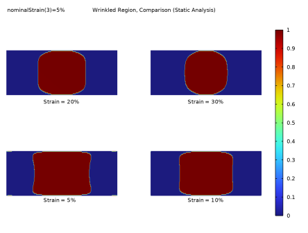
In the Settings window for 3D Plot Group, type Wrinkled Region, Comparison (Static Analysis) in the Label text field.
3
Locate the Data section. From the Dataset list, choose Layered Material 1.
4
From the Parameter value (nominalStrain (%)) list, choose 5.
5
Click to expand the Title section. From the Title type list, choose Label.
6
Locate the Plot Settings section. Clear the Plot dataset edges checkbox.
7
Click to expand the Plot Array section. From the Array type list, choose Square.
8
In the Relative row padding text field, type 0.5.
Surface 1
1
Right-click Wrinkled Region, Comparison (Static Analysis) and choose Surface.
2
In the Settings window for Surface, locate the Expression section.
3
In the Expression text field, type shell.syy<=0.
4
Click to expand the Quality section. From the Evaluation settings list, choose Manual.
5
From the Resolution list, choose No refinement.
6
From the Smoothing list, choose None.
Solution Array 1
1
Right-click Surface 1 and choose Solution Array.
2
In the Settings window for Solution Array, locate the Data section.
3
From the Parameter selection (nominalStrain) list, choose From list.
4
In the Parameter values (nominalStrain (%)) list, choose 5, 10, 20, and 30.
5
Locate the Plot Array section. From the Array shape list, choose Square.
Wrinkled Region, Comparison (Static Analysis)
In the Model Builder window, under Results click Wrinkled Region, Comparison (Static Analysis).
Table Annotation 1
1
In the Wrinkled Region, Comparison (Static Analysis) toolbar, click  More Plots and choose Table Annotation.
2
In the Settings window for Table Annotation, locate the Data section.
3
From the Source list, choose Local table.
4
5
Locate the Coloring and Style section. Clear the Show point checkbox.
Wrinkled Region, Comparison (Static Analysis)
1
Click the  Zoom Extents button in the Graphics toolbar.
2
In the Model Builder window, click Wrinkled Region, Comparison (Static Analysis).
3
In the Settings window for 3D Plot Group, locate the Plot Settings section.
4
From the View list, choose New view.
5
In the Wrinkled Region, Comparison (Static Analysis) toolbar, click  Plot.
6
Click the  Go to XY View button in the Graphics toolbar.
7
Click the  Show Grid button in the Graphics toolbar.
8
Click the  Show Axis Orientation button in the Graphics toolbar.
Transverse Stress, Longitudinal Line (Static Analysis)
1
In the Results toolbar, click  1D Plot Group.
2
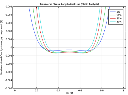
In the Settings window for 1D Plot Group, type Transverse Stress, Longitudinal Line (Static Analysis) in the Label text field.
3
Locate the Data section. From the Parameter selection (nominalStrain) list, choose Manual.
4
In the Parameter indices (1-13) text field, type 3,5,9,13.
5
Click to expand the Title section. From the Title type list, choose Label.
6
Locate the Axis section. Select the Manual axis limits checkbox.
7
In the x minimum text field, type -0.02.
8
In the x maximum text field, type 1.02.
9
In the y minimum text field, type -0.005.
10
In the y maximum text field, type 0.005.
Line Graph 1
1
Right-click Transverse Stress, Longitudinal Line (Static Analysis) and choose Line Graph.
2
3
In the Settings window for Line Graph, locate the y-Axis Data section.
4
In the Expression text field, type gpeval(4,shell.atxd1(0,mean(shell.syy)))/shell.Eequ.
5
Select the Description checkbox. In the associated text field, type Nondimensional Cauchy stress, yy component.
6
Locate the x-Axis Data section. From the Parameter list, choose Expression.
7
In the Expression text field, type X/L.
8
Click to expand the Legends section. Select the Show legends checkbox.
9
In the Transverse Stress, Longitudinal Line (Static Analysis) toolbar, click  Plot.
Transverse Stress, Transverse Line (Static Analysis)
1
In the Results toolbar, click  1D Plot Group.
2
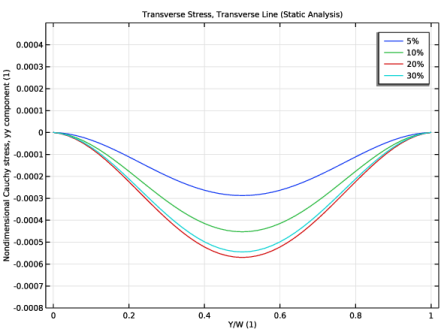
In the Settings window for 1D Plot Group, type Transverse Stress, Transverse Line (Static Analysis) in the Label text field.
3
Locate the Data section. From the Parameter selection (nominalStrain) list, choose Manual.
4
In the Parameter indices (1-13) text field, type 3,5,9,13.
5
Locate the Title section. From the Title type list, choose Label.
6
Locate the Axis section. Select the Manual axis limits checkbox.
7
In the x minimum text field, type -0.02.
8
In the x maximum text field, type 1.02.
9
In the y minimum text field, type -0.0008.
10
In the y maximum text field, type 0.0005.
Line Graph 1
1
Right-click Transverse Stress, Transverse Line (Static Analysis) and choose Line Graph.
2
3
In the Settings window for Line Graph, locate the y-Axis Data section.
4
In the Expression text field, type gpeval(4,shell.atxd1(0,mean(shell.syy)))/shell.Eequ.
5
Select the Description checkbox. In the associated text field, type Nondimensional Cauchy stress, yy component.
6
Locate the x-Axis Data section. From the Parameter list, choose Expression.
7
In the Expression text field, type Y/W.
8
Locate the Legends section. Select the Show legends checkbox.
9
In the Transverse Stress, Transverse Line (Static Analysis) toolbar, click  Plot.
Add Study
1
In the Home toolbar, click  Add Study to open the Add Study window.
2
Go to the Add Study window.
3
Find the Studies subsection. In the Select Study tree, select Preset Studies for Selected Physics Interfaces > Linear Buckling.
4
5
In the Home toolbar, click  Add Study to close the Add Study window.
Study: Prestressed Buckling Analysis
In the Settings window for Study, type Study: Prestressed Buckling Analysis in the Label text field.
Solution 2 (sol2)
In the Study toolbar, click  Show Default Solver.
Step 2: Linear Buckling
1
In the Model Builder window, under Study: Prestressed Buckling Analysis click Step 2: Linear Buckling.
2
In the Settings window for Linear Buckling, locate the Study Settings section.
3
In the Desired number of buckling modes text field, type 10.
4
Locate the Values of Linearization Point section. From the Settings list, choose User controlled.
5
From the Solution list, choose Solution 2 (sol2).
6
From the Use list, choose Solution Store 1 (sol3).
Solution 2 (sol2)
1
In the Model Builder window, expand the Study: Prestressed Buckling Analysis > Solver Configurations > Solution 2 (sol2) node.
2
In the Model Builder window, under Study: Prestressed Buckling Analysis > Solver Configurations > Solution 2 (sol2) click Eigenvalue Solver 1.
3
In the Settings window for Eigenvalue Solver, locate the General section.
4
In the Search for eigenfrequencies around shift text field, type 1.
5
From the Search method around shift list, choose Larger real part.
6
In the Study toolbar, click  Compute.
Results
Mode Shape (Prestressed Buckling Analysis)
1
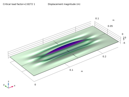
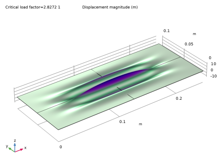
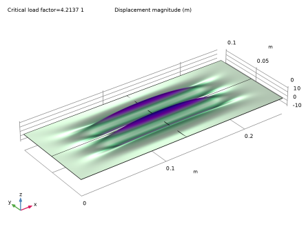
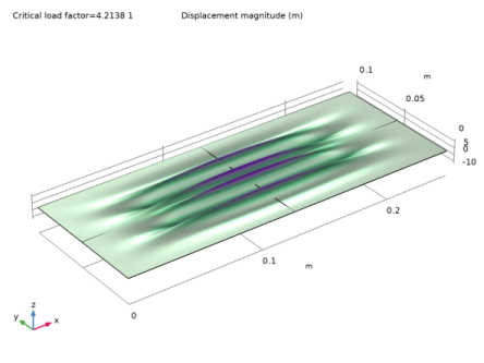
In the Settings window for 3D Plot Group, type Mode Shape (Prestressed Buckling Analysis) in the Label text field.
2
In the Mode Shape (Prestressed Buckling Analysis) toolbar, click  Plot.
Now, prescribe a deformation to the geometry from the calculated buckling modes to perform a postbuckling analysis.
Definitions (comp1)
Buckling Imperfection 1 (bcki1)
1
In the Definitions toolbar, click  Physics Utilities and choose Buckling Imperfection.
2
In the Settings window for Buckling Imperfection, locate the Deformed Geometry section.
3
Find the Mode selection subsection. In the table, enter the following settings:
4
Click Configure in the upper-right corner of the Deformed Geometry section. This creates a Prescribed Deformation node with the requested deformation settings. The newly created Prescribed Deformation node is automatically disabled in the existing study steps to enable further computations without changes in the results.
5
Locate the Nonlinear Buckling Study section. From the Load parameter list, choose nominalStrain.
6
From the Parameter value list list, choose User defined.
7
In the Range text field, type range(0,0.5,30).
8
In the Unit text field, type %.
9
Click Configure in the upper-right corner of the Nonlinear Buckling Study section.
This button creates a new study with stationary step, activates geometric nonlinearities and applies an auxiliary sweep for the postbuckling study.
Study: Postbuckling Analysis
1
In the Model Builder window, click Study 3.
2
In the Settings window for Study, locate the Study Settings section.
3
Clear the Generate default plots checkbox.
4
In the Label text field, type Study: Postbuckling Analysis.
5
In the Study toolbar, click  Compute.
Results
Layered Material 2
1
In the Results toolbar, click  More Datasets and choose Layered Material.
2
In the Settings window for Layered Material, locate the Data section.
3
From the Dataset list, choose Study: Postbuckling Analysis/Solution 4 (sol4).
Out-of-Plane Displacement, Comparison (Postbuckling)
1
In the Model Builder window, right-click Wrinkled Region, Comparison (Static Analysis) and choose Duplicate.
2
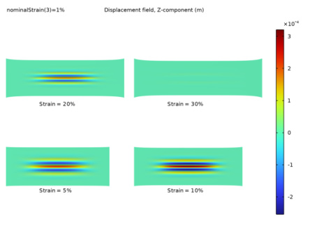
In the Settings window for 3D Plot Group, type Out-of-Plane Displacement, Comparison (Postbuckling) in the Label text field.
3
Locate the Data section. From the Dataset list, choose Layered Material 2.
4
Locate the Title section. From the Title type list, choose Automatic.
Surface 1
1
In the Model Builder window, expand the Out-of-Plane Displacement, Comparison (Postbuckling) node, then click Surface 1.
2
In the Settings window for Surface, locate the Expression section.
3
In the Expression text field, type w.
4
Locate the Quality section. From the Resolution list, choose Normal.
5
From the Smoothing list, choose Inside material domains.
Deformation 1
1
Right-click Surface 1 and choose Deformation.
2
In the Settings window for Deformation, locate the Expression section.
3
In the z-component text field, type w*10.
4
Locate the Scale section.
5
Select the Scale factor checkbox. In the associated text field, type 1.
Solution Array 1
1
In the Model Builder window, click Solution Array 1.
2
In the Settings window for Solution Array, locate the Data section.
3
In the Parameter values (nominalStrain (%)) list, choose 5, 10, 20, and 30.
Out-of-Plane Displacement, Comparison (Postbuckling)
1
In the Model Builder window, under Results click Out-of-Plane Displacement, Comparison (Postbuckling).
2
In the Out-of-Plane Displacement, Comparison (Postbuckling) toolbar, click  Plot.
Out-of-Plane Displacement, Comparison (Postbuckling) 1
Right-click Out-of-Plane Displacement, Comparison (Postbuckling) and choose Duplicate.
Surface 1
1
In the Model Builder window, expand the Out-of-Plane Displacement, Comparison (Postbuckling) 1 node.
2
In the Model Builder window, expand the Surface 1 node.
Solution Array 1, Table Annotation 1
1
In the Model Builder window, under Results > Out-of-Plane Displacement, Comparison (Postbuckling) 1, Ctrl-click to select Surface 1 > Solution Array 1 and Table Annotation 1.
2
Out-of-Plane Displacement (Postbuckling)
1
In the Model Builder window, under Results click Out-of-Plane Displacement, Comparison (Postbuckling) 1.
2
In the Settings window for 3D Plot Group, type Out-of-Plane Displacement (Postbuckling) in the Label text field.
3
Locate the Plot Settings section. From the View list, choose New view.
4
In the Out-of-Plane Displacement (Postbuckling) toolbar, click  Plot.
5
Click the  Go to XY View button in the Graphics toolbar.
6
Click the  Show Axis Orientation button in the Graphics toolbar.
7
Click the  Show Grid button in the Graphics toolbar.
Animation: Out-of-Plane Displacement (Postbuckling)
1
In the Results toolbar, click  Animation and choose Player.
2
In the Settings window for Animation, type Animation: Out-of-Plane Displacement (Postbuckling) in the Label text field.
3
Locate the Scene section. From the Subject list, choose Out-of-Plane Displacement (Postbuckling).
4
Locate the Playing section. In the Display each frame for text field, type 0.2.
5
Click  Show Frame.
Wrinkle Amplitude (Postbuckling)
1
In the Results toolbar, click  1D Plot Group.
2
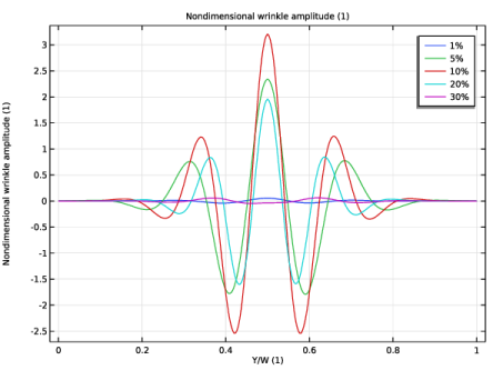
In the Settings window for 1D Plot Group, type Wrinkle Amplitude (Postbuckling) in the Label text field.
3
Locate the Data section. From the Dataset list, choose Study: Postbuckling Analysis/Solution 4 (sol4).
4
From the Parameter selection (nominalStrain) list, choose Manual.
5
In the Parameter indices (1-61) text field, type 3,11,21,41,61.
Line Graph 1
1
Right-click Wrinkle Amplitude (Postbuckling) and choose Line Graph.
2
3
In the Settings window for Line Graph, locate the y-Axis Data section.
4
In the Expression text field, type w/th.
5
Select the Description checkbox. In the associated text field, type Nondimensional wrinkle amplitude.
6
Locate the x-Axis Data section. From the Parameter list, choose Expression.
7
In the Expression text field, type Y/W.
8
Locate the Legends section. Select the Show legends checkbox.
9
In the Wrinkle Amplitude (Postbuckling) toolbar, click  Plot.
Wrinkle Amplitude vs. Nominal Strain (Postbuckling)
1
In the Results toolbar, click  1D Plot Group.
2
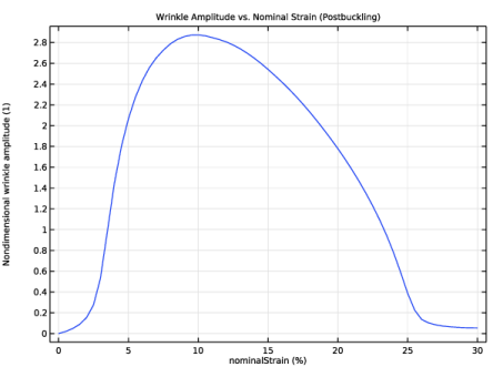
In the Settings window for 1D Plot Group, type Wrinkle Amplitude vs. Nominal Strain (Postbuckling) in the Label text field.
3
Locate the Title section. From the Title type list, choose Label.
4
Locate the Data section. From the Dataset list, choose Study: Postbuckling Analysis/Solution 4 (sol4).
Point Graph 1
1
Right-click Wrinkle Amplitude vs. Nominal Strain (Postbuckling) and choose Point Graph.
2
3
In the Settings window for Point Graph, locate the y-Axis Data section.
4
In the Expression text field, type 0.5*(maxop1(w)-minop1(w))/th.
5
Select the Description checkbox. In the associated text field, type Nondimensional wrinkle amplitude.
6
In the Wrinkle Amplitude vs. Nominal Strain (Postbuckling) toolbar, click  Plot.
Study: Static Analysis
Step 1: Stationary
In Study 1: Static Analysis, disable the Prescribed Deformation node.
1
In the Model Builder window, under Study: Static Analysis click Step 1: Stationary.
2
In the Settings window for Stationary, locate the Physics and Variables Selection section.
3
Select the Modify model configuration for study step checkbox.
4
In the tree, select Component 1 (comp1) > Deformed Geometry, Controls material frame > Prescribed Deformation, Shell.
5