|
|
|
|
•
|
|
•
|
|
•
|
Murnaghan third-order elastic constants: l = −24.8·1010 Pa, m = −62.3·1010 Pa, and n = −71.4·1010 Pa.
|
|
1
|
|
2
|
|
3
|
Click Add.
|
|
4
|
Click
|
|
5
|
|
6
|
Click
|
|
1
|
|
2
|
|
1
|
|
2
|
|
3
|
|
4
|
|
5
|
|
6
|
Click
|
|
7
|
|
1
|
|
2
|
|
1
|
|
2
|
|
3
|
|
4
|
|
1
|
In the Model Builder window, under Component 1 (comp1) right-click Materials and choose Blank Material.
|
|
2
|
|
1
|
|
1
|
|
3
|
|
4
|
|
5
|
|
1
|
|
2
|
|
3
|
|
1
|
|
3
|
|
1
|
|
2
|
|
1
|
|
1
|
|
2
|
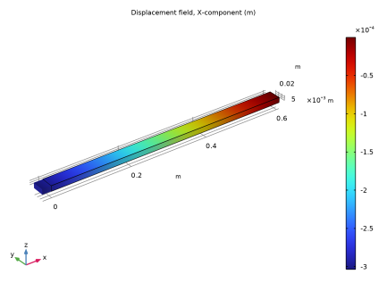
In the Settings window for Surface, click Replace Expression in the upper-right corner of the Expression section. From the menu, choose Component 1 (comp1) > Solid Mechanics > Displacement > Displacement field - m > u - Displacement field, X-component.
|
|
3
|
|
1
|
|
2
|
Go to the Add Study window.
|
|
3
|
Find the Studies subsection. In the Select Study tree, select Preset Studies for Selected Physics Interfaces > Eigenfrequency, Prestressed.
|
|
4
|
Click the Add Study button in the window toolbar.
|
|
5
|
|
1
|
|
2
|
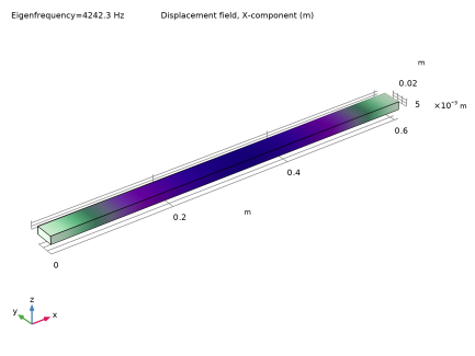
In the Settings window for Surface, click Replace Expression in the upper-right corner of the Expression section. From the menu, choose Component 1 (comp1) > Solid Mechanics > Displacement > Displacement field - m > u - Displacement field, X-component.
|
|
3
|
|
1
|
|
2
|
|
3
|
|
1
|
|
2
|
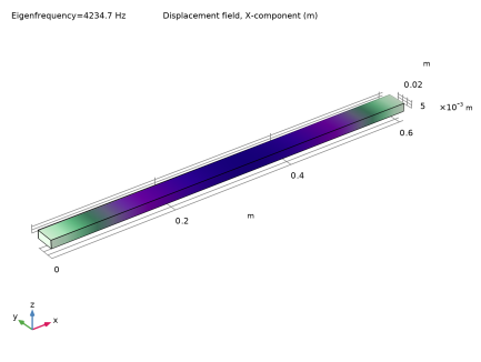
In the Settings window for Surface, click Replace Expression in the upper-right corner of the Expression section. From the menu, choose Component 1 (comp1) > Solid Mechanics > Displacement > Displacement field - m > u - Displacement field, X-component.
|
|
1
|
|
2
|
|
3
|