
|
|
|


|
1
|
|
2
|
|
3
|
Click Add.
|
|
4
|
Click
|
|
5
|
|
6
|
Click
|
|
1
|
|
2
|
|
1
|
|
2
|
|
3
|
|
4
|
|
5
|
|
6
|
|
7
|
Click
|
|
8
|
|
1
|
|
2
|
|
1
|
|
1
|
|
1
|
|
3
|
|
4
|
|
1
|
|
2
|
In the Settings window for Hyperelastic Material, type Polynomial, Two Parameters in the Label text field.
|
|
3
|
|
4
|
|
5
|
|
6
|
|
7
|
|
1
|
|
1
|
|
3
|
|
4
|
|
5
|
|
6
|
|
7
|
Select the Reverse direction checkbox.
|
|
1
|
|
3
|
|
4
|
|
5
|
|
6
|
|
1
|
|
2
|
|
3
|
|
4
|
|
5
|
|
6
|
Click
|
|
1
|
|
2
|
|
3
|
|
4
|
Locate the Hyperelastic Material section. From the Material model list, choose Mooney–Rivlin, two parameters.
|
|
5
|
|
6
|
|
7
|
|
1
|
|
2
|
In the Settings window for Hyperelastic Material, type Polynomial, Five Parameters in the Label text field.
|
|
3
|
|
1
|
|
2
|
|
1
|
|
2
|
|
3
|
Select the Modify model configuration for study step checkbox.
|
|
4
|
In the tree, select Component 1 (comp1) > Solid Mechanics (solid), Controls spatial frame > Mooney–Rivlin and Component 1 (comp1) > Solid Mechanics (solid), Controls spatial frame > Polynomial, Five Parameters.
|
|
5
|
Click
|
|
6
|
|
1
|
|
2
|
|
3
|
Click
|
|
4
|
|
5
|
Click OK.
|
|
6
|
|
8
|
Click
|
|
1
|
|
2
|
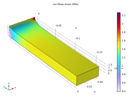
In the Settings window for 3D Plot Group, type Stress (Polynomial, Two Parameters) in the Label text field.
|
|
1
|
In the Model Builder window, expand the Stress (Polynomial, Two Parameters) node, then click Volume 1.
|
|
2
|
|
3
|
|
1
|
|
2
|
|
3
|
|
4
|
Click Replace Expression in the upper-right corner of the Expressions section. From the menu, choose Component 1 (comp1) > Solid Mechanics > Displacement > Displacement field - m > v - Displacement field, Y-component.
|
|
5
|
|
6
|
Click
|
|
1
|
|
2
|
Go to the Add Study window.
|
|
3
|
|
4
|
Click the Add Study button in the window toolbar.
|
|
5
|
|
1
|
|
2
|
Select the Modify model configuration for study step checkbox.
|
|
3
|
In the tree, select Component 1 (comp1) > Solid Mechanics (solid), Controls spatial frame > Polynomial, Five Parameters.
|
|
4
|
Click
|
|
5
|
|
6
|
|
7
|
|
1
|
|
2
|
|
3
|
|
1
|
|
2
|
|
3
|
|
4
|
Click
|
|
1
|
|
2
|
Go to the Add Study window.
|
|
3
|
|
4
|
Click the Add Study button in the window toolbar.
|
|
5
|
|
1
|
|
2
|
|
1
|
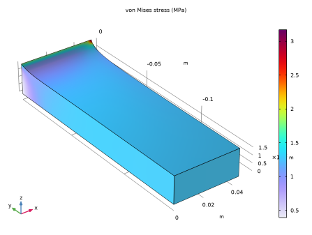
In the Model Builder window, expand the Stress (Polynomial, Five Parameters) node, then click Volume 1.
|
|
2
|
|
3
|
|
1
|
|
2
|
|
3
|
|
4
|
Click
|
|
1
|
|
2
|
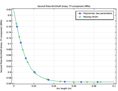
In the Settings window for 1D Plot Group, type Second Piola-Kirchhoff Stress in the Label text field.
|
|
1
|
|
3
|
In the Settings window for Line Graph, click Replace Expression in the upper-right corner of the y-Axis Data section. From the menu, choose Component 1 (comp1) > Solid Mechanics > Stress > Second Piola–Kirchhoff stress (material and geometry frames) - N/m² > solid.SGpYY - Second Piola–Kirchhoff stress, YY-component.
|
|
4
|
Click to expand the Coloring and Style section. Find the Line markers subsection. From the Marker list, choose Cycle.
|
|
5
|
|
6
|
|
7
|
|
1
|
|
2
|
|
3
|
|
4
|
Locate the Coloring and Style section. Find the Line markers subsection. In the Number text field, type 10.
|
|
5
|
Locate the Legends section. In the table, enter the following settings:
|
|
6
|
|
7
|